FINAL PROJECT: Design of Electric Vehicle

Create a MATLAB model of electric car which uses a battery and a DC motor. Choose suitable blocks from Powertrain block set. Prepare a report about your model including following:

Objectives:

1. System level configurations
2. Model parameters
3. Results
4. Conclusion

Electric Car Components and Functions

Electric Car Components

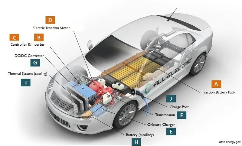
Electric car or vehicle component and function depend on the car type. There are at least four types of electric cars currently sold commercially and operates in the world. Here,we will discuss various common main electric car components or parts or elements and their function such as traction batteries, inverters (DC-DC converters), traction motors, on-board chargers and controllers. The different types of electric car components determines how the car works. Electric cars (vehicles) components and functions can be explained by means of picture below.

———————————————

How Does An Electric Car Work?

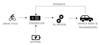
When the car pedal is pressed, then:

• Controller [C] takes and regulates electrical energy from batteries [A] and inverters [B]
• With the controller set, the inverter then sends a certain amount of electrical energy to the motor (according to the depth of pressure on the pedal)
• Electric motor [D] converts electrical energy into mechanical energy (rotation)
• Rotation of the motor rotor rotates the transmission so the wheels turn and then the car moves.

Note: The working principle above is for battery electric vehicle (BEV) type.

———————————————

Electric Vehicle Components

Basic Main Components of Electrical Vehicle

The basic main elements of electric cars installed in almost all types of electric cars are as follows:

Traction Battery Pack (A)

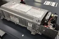
The function of the battery in an electric car is as an electrical energy storage system in the form of direct-current electricity (DC). If it gets a signal from the controller, the battery will flow DC electrical energy to the inverter to then be used to drive the motor. The type of battery used is a rechargeable battery that is arranged in such a way as to form what is called a traction battery pack.

There are various types of electric car batteries. The most widely used is the type of lithium-ion batteries.

Power Inverter (B)

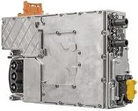
The inverter functions to change the direct current (DC) on the battery into an alternating current (AC) and then this alternating current is used by an electric motor. In addition, the inverter on an electric car also has a function to change the AC current when regenerative braking to DC current and then used to recharge the battery. The type of inverter used in some electric car models is the bi-directional inverter category.

Controller (C)

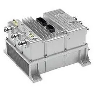
The main function of the controller is as a regulator of electrical energy from batteries and inverters that will be distributed to electric motors. While the controller itself gets the main input from the car pedal (which is set by the driver). This pedal setting will determine the frequency variation or voltage variation that will enter the motor, and at the same time determine the car’s speed.

In brief, this unit manages the flow of electrical energy delivered by the traction battery, controlling the speed of the electric traction motor and the torque it produces. This component will determine how electric car work.

Electric Traction Motor (D)

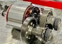
Because the controller provides electrical power from the traction battery, the electric traction motors will work turning the transmission and wheels. Some hybrid electric cars use a type of generator-motor that performs the functions of propulsion and regeneration. In general, the type of electric motor used is the BLDC (brushless DC) motor

———————————————

Other Electric Car Components

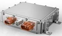
Charger (E) is a battery charging device. Chargers get electricity from outside sources, such as the utility grid or solar power plants. AC electricity is converted into DC electricity and then stored in the battery. There are 2 types of electric car chargers:

• On-board charger: the charger is located and installed in the car
• Off-board charger: the charger is not located or not installed in the car.

Transmission (F): The transmission transfers mechanical power from the electric traction motor to drive the wheels.

DC/DC Converter (G): This one of electric car parts that to converts higher-voltage DC power from the traction battery pack to the lower-voltage DC power needed to run vehicle accessories and recharge the auxiliary battery.

Battery (H): In an electric drive vehicle, the auxiliary battery provides electricity to power vehicle accessories.

Thermal System – Cooling (I): This system maintains a proper operating temperature range of the engine, electric motor, power electronics, and other components.

Charge Port (J): The charge port allows the vehicle to connect to an external power supply in order to charge the traction battery pack.

BLOCK DIAGRAM OF ELECTRIC VEHICLES:

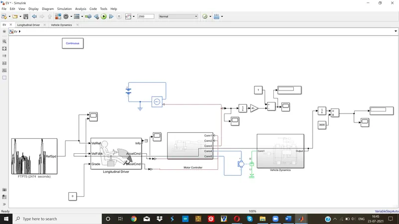
MATLAB SIMULATION MODEL:

Vehicle Dynamics subsystem:

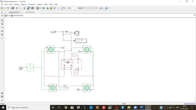
Vehicle dynamics subsystem consists of :

• Vehicle body
• Tires
• Simple gear
• Terminator
• Scope
• Display
• Constant blocks

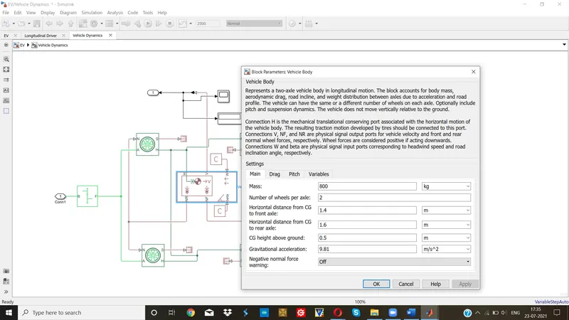
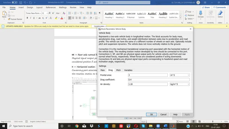
1. Vehicle Body-

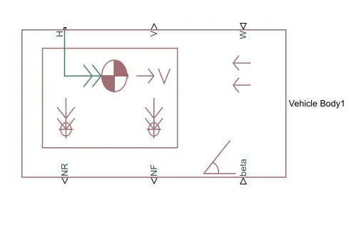
The Vehicle Body block represents a two-axle vehicle body in longitudinal motion. The vehicle can have the same or a different number of wheels on each axle. For example, two wheels on the front axle and one wheel on the rear axle. The vehicle wheels are assumed identical in size. The vehicle can also have a center of gravity (CG) that is at or below the plane of travel.

The block accounts for body mass, aerodynamic drag, road incline, and weight distribution between axles due to acceleration and road profile. Optionally include pitch and suspension dynamics. The vehicle does not move vertically relative to the ground.

The block has an option to include an externally-defined mass and an externally-defined inertia. The mass, inertia, and center of gravity of the vehicle body can vary over the course of simulation in response to system changes.

W — Headwind speed, m/s

Physical signal input port for headwind speed.

beta — Road incline angle, rad

Physical signal input port for road incline angle.

CG — Center of gravity, m

Physical signal input port for the center of gravity, in m, of the externally-defined mass relative to the CG of the vehicle body.

M — Mass, kg

Physical signal input port for the mass, in kg, of the externally-defined mass.

J — External moment of inertia, kg*m^2

Physical signal input port for the moment of inertia, in kg*m^2, of the externally-defined mass.

V — Longitudinal velocity, m/s

Physical signal output port for vehicle longitudinal velocity.

NF — Front axle normal force, N

Physical signal output port for normal force on the front axle. Wheel forces are considered positive if acting downwards.

NR — Rear axle normal force, N

Physical signal output port for normal force on the rear axle. Wheel forces are considered positive if acting downwards.

H — Horizontal motion

Conserving port associated with the horizontal motion of the vehicle body. Connect tire traction motion to this port.

2. Tire(Magic formula)-

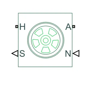
The Tire (Magic Formula) block models a tire with longitudinal behavior given by the Magic Formula [1], an empirical equation based on four fitting coefficients. The block can model tire dynamics under constant or variable pavement conditions.

The longitudinal direction of the tire is the same as its direction of motion as it rolls on pavement.

A — Axle:

Mechanical rotational port associated with the axle that the tire sits on.

H — Hub

Mechanical translational port associated with the wheel hub that transmits the thrust generated by the tire to the remainder of the vehicle.

N — Normal force

Physical signal input port associated with the normal force acting on the tire. The normal force is positive if it acts downward on the tire, pressing it against the pavement.

S — Slip (Output)

Physical signal output port associated with the relative slip between the tire and road.

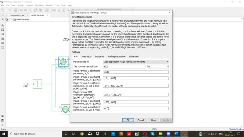
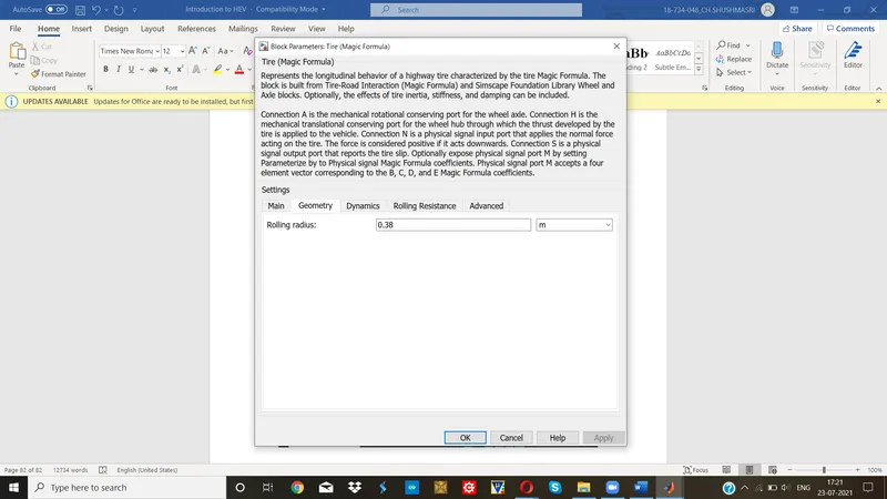
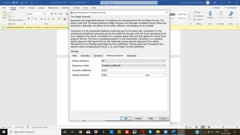
3. Simple gear:

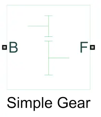
The Simple Gear block represents a gearbox that constrains the connected driveline axes of the base gear, B, and the follower gear, F, to corotate with a fixed ratio that you specify. We can choose whether the follower axis rotates in the same or opposite direction as the base axis. If they rotate in the same direction, the angular velocity of the follower, ω_F, and the angular velocity of the base, ω_B, have the same sign. If they rotate in opposite directions, ω_F and ω_B have opposite signs.

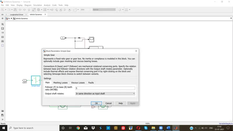
EXPLANATION FOR VEHICLE BODY SUBSYSTEM:

• Transmission system procides propulsion power from motor to wheels, hence, this is very important component of vehicle.
• The basic components required in a vehicle are: simple gear, Vehicle body, Tires.
• Tire block is fed with the existing tire parameters. According to the requirements, the parameters are given.
• The four tires are placed in the model. The first two tires in the model are Rear wheels andd the other two are Front wheels.
• Axle is connected for first two tyres and also connect other two tyres. H ports of all the tyres are connected. N of rear tires are connected to NR and N of rear tires are connected to NF of Vehicle body.S are not used so, connect them to terminator.
• W and BETA port are wind speed and inclination angle. These can be given using PS constant blocks. In the model, the values considered for W and BETA are 4 and 0 respectively.
• Velocity is the output of this subsystem hence, it is connected to output port. The power transmitted from motor to rear wheels using simple gear. As power is transmitted to rear wheels, the model is considered as rear wheel drive.
• Hence, subsytem is modelled where input is power from motor and output is velocity with which vehicle moves.

Motor controller subsystem:

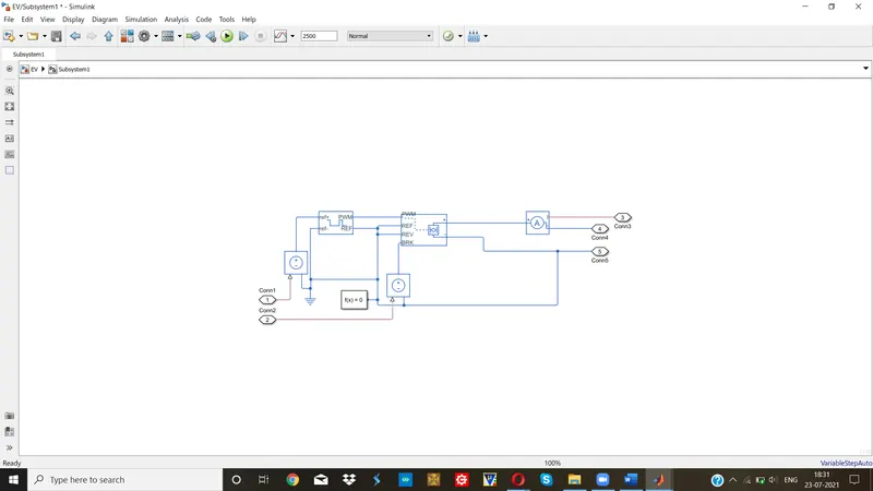
The following components are used to model the motor controller subsystem:

• H-bridge
• Controlled PWM Voltage
• Controlled voltage source
• Current sensor
• Solver configuration
• Electrical reference

1. H-bridge:

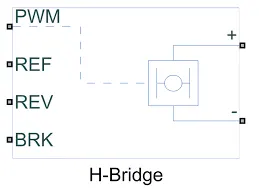
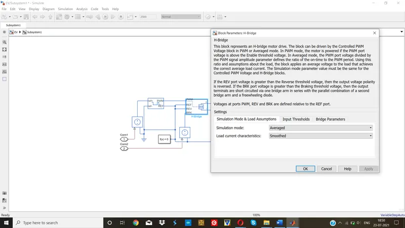
The H-Bridge block represents an H-bridge motor driver. The block has the following two Simulation mode options:

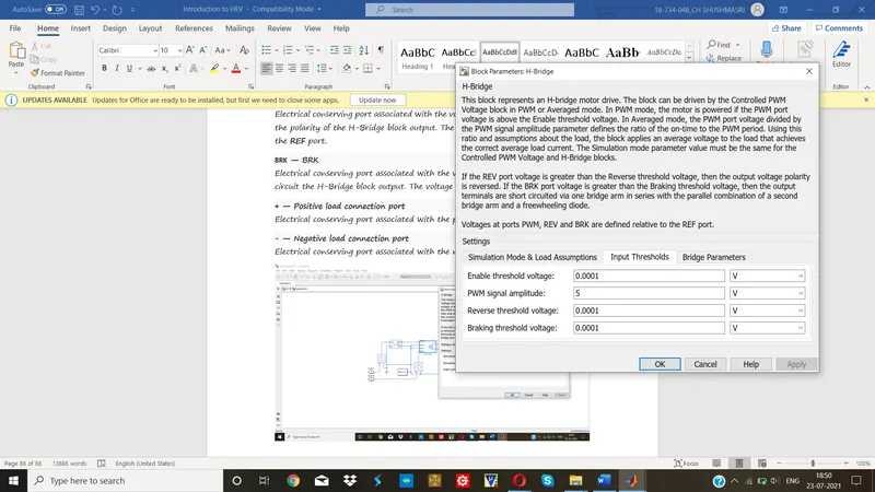
• PWM— The H-Bridge block output is a controlled voltage that depends on the input signal at the PWM If the input signal has a value greater than the Enable threshold voltage parameter value, the H-Bridge block output is on and has a value equal to the value of the Output voltage amplitude parameter. If it has a value less than the Enable threshold voltage parameter value, the block maintains the load circuit using one of the following three Freewheeling mode options:
  • Via one semiconductor switch and one freewheeling diode
  • Via two freewheeling diodes
  • Via two semiconductor switches and one freewheeling diode

The first and third options are sometimes referred to as synchronous operation.

The signal at the REV port determines the polarity of the output. If the value of the signal at the REV port is less than the value of the Reverse threshold voltage parameter, the output has positive polarity; otherwise, it has negative polarity.

• Averaged— This mode has two Load current characteristics options:
  • Smoothed
  • Unsmoothed or discontinuous

The Smoothed option assumes that the current is practically continuous due to load inductance.

where:

• V_Ois the value of the Output voltage amplitude
• V_PWMis the value of the voltage at the PWM
• A_PWMis the value of the PWM signal amplitude
• I_OUTis the value of the output current.
• R_ONis the Bridge on resistance

The current will be smooth if the PWM frequency is large enough. Synchronous operation where freewheeling is via a bridge arm back to the supply also helps smooth the current. For cases where the current is not smooth, or possibly discontinuous (that is, it goes to zero between PWM cycles), use the Unsmoothed or discontinuous option. For this option, you must also provide values for the Total load series resistance, Total load series inductance, and PWM frequency. During simulation, the block uses these values to calculate a more accurate value for H-bridge output voltage that achieves the same average current as would be present if simulating in PWM mode.

PWM — Pulse-width modulated signal

Electrical conserving port associated with the pulse-width modulated signal. The voltage is defined relative to the REF port.

REF — Reference

Electrical conserving port associated with the floating zero volt reference.

REV — REV

Electrical conserving port associated with the voltage that controls when to reverse the polarity of the H-Bridge block output. The voltage is defined relative to the REF port.

BRK — BRK

Electrical conserving port associated with the voltage that controls when to short circuit the H-Bridge block output. The voltage is defined relative to the REF port.

+ — Positive load connection port

Electrical conserving port associated with the positive load connection.

- — Negative load connection port

Electrical conserving port associated with the negative load connection.

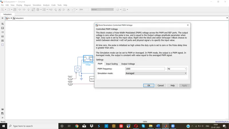
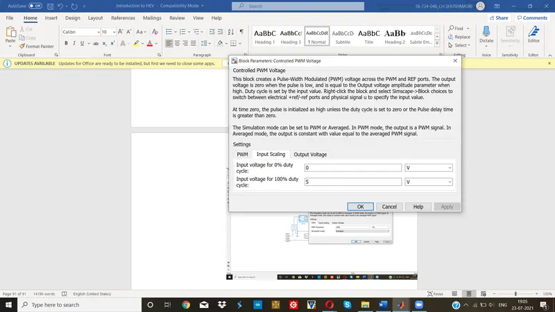
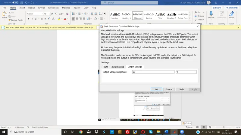
2. Controlled PWM voltage:

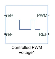
The Controlled PWM Voltage block represents a pulse-width modulated (PWM) voltage source. The block has two modeling variants, accessible by right-clicking the block in your block diagram and then selecting the appropriate option from the context menu, under Simscape > Block choices:

• Electrical input ports— The block calculates the duty cycle based on the reference voltage across its ref+ and ref- This modeling variant is the default.
• PS input— Specify the duty cycle value directly by using an input physical signal port.

In PWM mode, the block has two options for the type of switching event when moving between output high and output low states:

• Asynchronous – Best for variable-step solvers— Asynchronous events are better suited to variable step solvers, because they require fewer simulation steps for the same level of accuracy. In asynchronous mode the PWM switching events generate zero crossings, and therefore switching times are always determined accurately, regardless of the simulation maximum step size.
• Discrete—time – Best for fixed-step solvers— Discrete-time events are better suited to fixed-step operation, because then the switching events are always synchronized with the simulation step. Using an asynchronous implementation with fixed-step solvers may sometimes result in events being up to one simulation step late.

If you use a fixed-step or local solver and the discrete-time switching event type, the following restrictions apply to the Sample time parameter value:

• The sample time must be a multiple of the simulation step size.
• The sample time must be small compared to the PWM period, to ensure sufficient resolution.

ref+ — Positive terminal

Positive electrical reference voltage.

ref- — Negative terminal

Negative electrical reference voltage

PWM — Pulse-width modulated signal

Electrical conserving port associated with the pulse-width modulated signal.

REF — Floating zero volt reference

Electrical conserving port associated with the floating zero volt reference.

3. Controlled Voltage source:

The Controlled Voltage Source block represents an ideal voltage source that is powerful enough to maintain the specified voltage at its output regardless of the current flowing through the source.

The output voltage is V = Vs, where Vs is the numerical value presented at the physical signal port.

The block has one physical signal input port and two electrical conserving ports associated with its electrical terminals.

4. Current sensor:

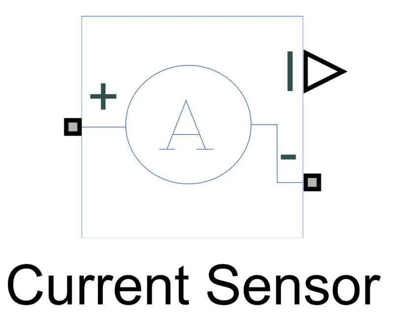
The Current Sensor block represents an ideal current sensor, that is, a device that converts current measured in any electrical branch into a physical signal proportional to the current.

Connections + and – are electrical conserving ports through which the sensor is inserted into the circuit. Connection I is a physical signal port that outputs the measurement result.

The block has the following ports:

+

Electrical conserving port associated with the sensor positive terminal.

-

Electrical conserving port associated with the sensor negative terminal.

I

Physical signal output port for current.

5. Solver configuration:

Each physical network represented by a connected Simscape™ block diagram requires solver settings information for simulation. The Solver Configuration block specifies the solver parameters that your model needs before you can begin simulation.

Each topologically distinct Simscape block diagram requires exactly one Solver Configuration block to be connected to it.

The block has one conserving port. We can add this block anywhere on a physical network circuit by creating a branching point and connecting it to the only port of the Solver Configuration block.

6. Scope:

Scope is used to view the waveforms at certain point.

EXPLANATION FOR MOTOR CONTROLLER SYSTEM:

• The main components of motor controller system comprises of H-bridge, Controlled PWM Voltage.
• Controller is used to get output according to the requirement.
• H-bridge provides supply to the motor from DC battery supply.
• H-bridge parameters contains two simulation types- averaged or PWM. In this model, averaged simulation is done so as to reduce the simulation time.
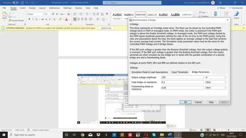
• The output of H-bridge is same as the rated input of DC motor used.
• There is a PWM signal port in H- bridge to which controlled PWM voltage is given. The REV and REF are connected to electrical ground in order to avoid reverse operation of motor. The BRK port is connected to controlled voltage source such that regenerative braking can be performed. This represents Wide Open Throttle of brake pedal.
• PWM port of Controlled PWM voltage is connected to PWM port of H-bridge. The -ve Reference is grounded as negative voltages are not required. The +ve Reference is connected to Controlled Voltage source.
• This subsystem creates pulses from DC supply, which drives the motor. By changing the voltage of battery, the speed and frequency of motor can be changed.
• This subsystem controls the power of the motor.

Distance Calculation:

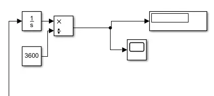
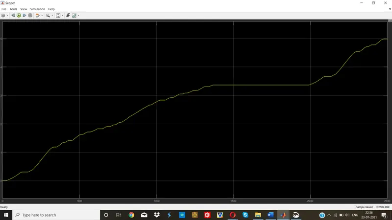
The speed is divided by 3600 to convert velocity from km/hr to km/s. Then the resultant is integrated to get distance in km. The waveform of distance can be viewed using scope and overall distance can be seen in the display.

State of charge calculation:

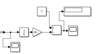
The components used here are:

• Integrator
• Gain
• Add
• Constant
• Scope
• Display

1. Integrator:

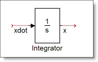
Integrator gives integration of input signal with respect to time.

2. Gain

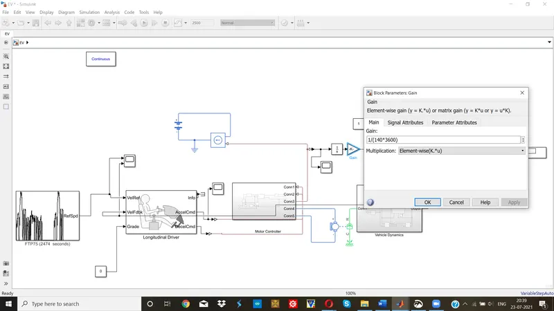
The Gain block multiplies the input by a constant value (gain). The input and the gain can each be a scalar, vector, or matrix.

EXPLANATION FOR SOC CALCULATION:

• SOC calculation uses an integrator, gain, adder, scope, display.
• Integrator block gives the integration of velocity signal and then gain block is connected to it.
• Gain block divides the present signal by product of 14oAH which is the amp hour rating of battery and 3600 to convert hours in seconds.
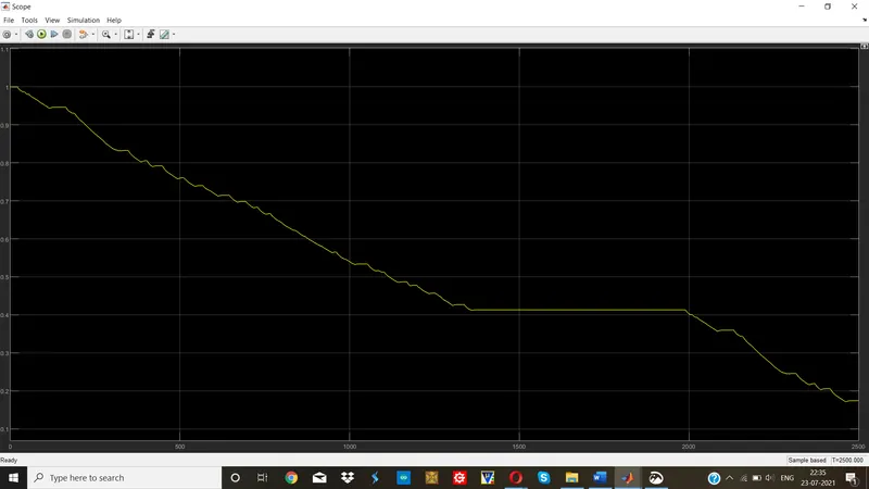
• Constant block is used to represent initial state of charge of the battery. In the model initial state of charge is assumed to be 1 which denotes 100% charging.
• Sum block performs addition or subtraction of the signals.

Drive cycle source:

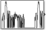
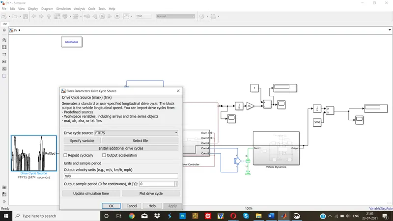
The Drive Cycle Source block generates a standard or user-specified longitudinal drive cycle. The block output is the specified vehicle longitudinal speed, which you can use to:

• Predict the engine torque and fuel consumption that a vehicle requires to achieve desired speed and acceleration for a given gear shift reference.
• Produce realistic velocity and shift references for closed loop acceleration and braking commands for vehicle control and plant models.
• Study, tune, and optimize vehicle control, system performance, and system robustness over multiple drive cycles.

Drive cycles from predefined sources. By default, the block includes the FTP–75 drive cycle.

Longitudinal driver:

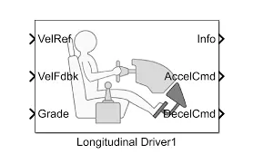
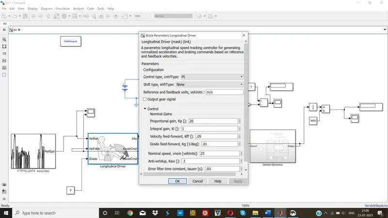
The Longitudinal Driver block implements a longitudinal speed-tracking controller. Based on reference and feedback velocities, the block generates normalized acceleration and braking commands that can vary from 0 through 1. You can use the block to model the dynamic response of a driver or to generate the commands necessary to track a longitudinal drive cycle.

Battery:

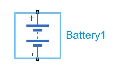
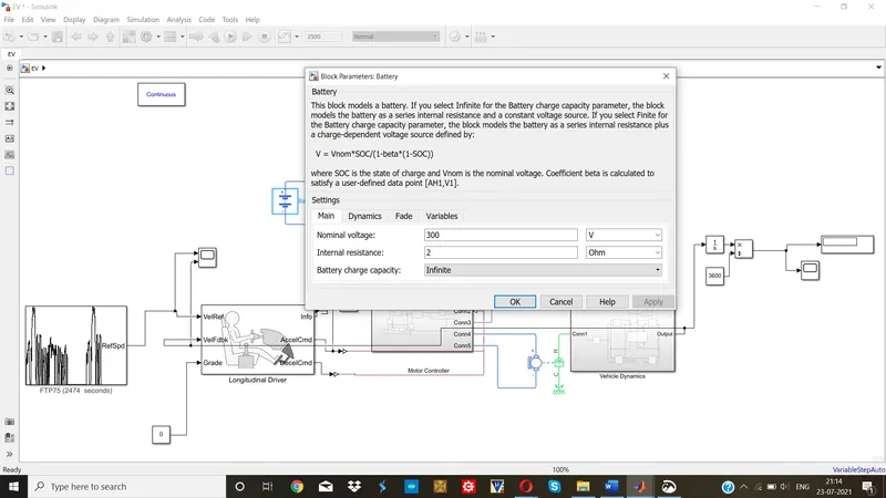
The Battery block represents a simple battery model. The block has four modeling variants, accessible by right-clicking the block in your block diagram and then selecting the appropriate option from the context menu, under Simscape > Block choices:

• Uninstrumented | No thermal port— Basic model that does not output battery charge level or simulate thermal effects. This modeling variant is the default.
• Uninstrumented | Show thermal port— Model with exposed thermal port. This model does not measure internal charge level of the battery.
• Instrumented | No thermal port— Model with exposed charge output port. This model does not simulate thermal effects.
• Instrumented | Show thermal port— Model that lets you measure internal charge level of the battery and simulate thermal effects. Both the thermal port and the charge output port are exposed.

Controlled current source:

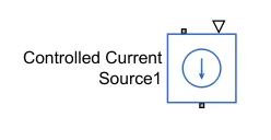
The Controlled Current Source block represents an ideal current source that is powerful enough to maintain the specified current through it regardless of the voltage across the source.

The output current is I = Is, where Is is the numerical value presented at the physical signal port.

The positive direction of the current flow is indicated by the arrow.

The block has one physical signal input port and two electrical conserving ports associated with its electrical terminals.

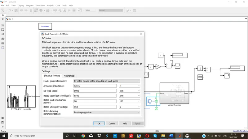
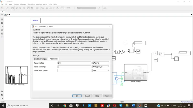
DC motor:

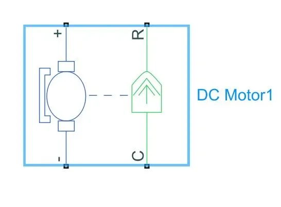
The DC Motor block represents the electrical and torque characteristics of a DC motor using the following equivalent circuit model:

You specify the equivalent circuit parameters for this model when you set the Model parameterization parameter to By equivalent circuit parameters. The resistor R corresponds to the resistance you specify in the Armature resistance parameter. The inductor L corresponds to the inductance you specify in the Armature inductance parameter.

Display:

The Display block shows the value of the input data. We can specify the frequency of the display. We can also specify the format of display.

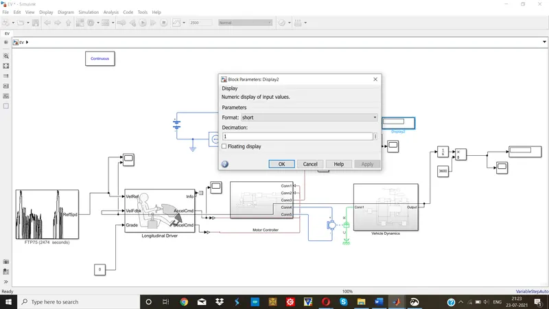
EXPLANATION OF THE MODEL:

• Appropriate motor is selected and based on the requirement of speed, DC supply voltage is adjusted.
• Motor block has 4 ports: +,- C,R. C is considered to be non- rotating hence, it is given to mechanical reference. + and – are power supply terminals.
• Port-R is connected to simple gear in vehicle dynamics subsystem.
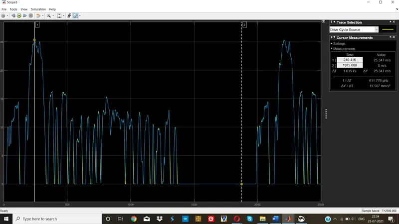
• In longitudinal friver, Drive cycle is connected to VelRef and VelFdbk comes from vehicle dynamics. These both signals are compared. When VelFdbk is greater than VelRef, deceleration command is sent which can be seen in DecelCmd and when VelFdbk is lesser than VelRef acceleration comman is sent which is seen in AccelCmd port.
• The graph of speed of the standard drive cycle and speed with which vehicle moves which is an output of Vehicle Dynamics block are obtained in single scope so that both the graphs can be compared.
• Area under the velocity-time graph gives distance. The integration of velocity with respect to time in hours gives distance. To get time in hours, we divide it which 3600.
• Finally, simulation is done for simulation time of 2500s.

RESULTS:

Drive cycle	FTP75
Distance (km)	4.982
Top speed(m/s)	25.347
Simulation time (s)	2500
Vehicle weight(kg)	800
Frontal area (m^2)	3
Drag coefficient	0.4
Battery nominal voltage(V)	300
DC motor rated load(kW)	60
DC motor rated voltage(V)	150
H-bridge output voltage(V)	150
SOC at the end of simulation (%)	17.4
Top speed reached ?	YES

OUTPUT GRAPH:

SPEED GRAPH

SOC

DISTANCE:

CONCLUSION:

• From the graphs above, we observe that the feedback speed plot and reference speed plot overlap with each other at most of the times. They are not equal whenever the vehicle starts to decelerate.
• In SOC plot, we observe that State of charge decreases when acceleration takes place and when deceleration is happening, the State of Charge increases due to regenerative braking.
• In distance graph, we observe that whenever acceleration is taking place, the slope increases and when deceleration takes place, the slope deceases.

https://drive.google.com/file/d/1LfWERTJTsVql4RDYv9zr13G6dxZ5sWBA/view?usp=sharing