FINAL INDEPENDENT PROJECT
Robotics with Matlab: Direct Kinematics and Simulation
Abstract: This paper introduces to implementation and understanding of the bases of simulation models for the study of the movement of the different types of robots. We will implement simulation models of mobile platforms such as the unidirectional cycle of three wheels four wheels type Mecano and other settings. We will also review robotic arms aerial robots that in the end, we will combine these robotic systems to train new ones like mobile manipulators and aerial manipulators. It will be using these models to perform control algorithms such as position control without with orientation trajectory following control road the following control and it will also be seen cooperative control and many more algorithms.
Introduction
The direct kinematics of a robot is kinematics because it is the study of movements of a robot. It is calculated the position, speed, and acceleration at a point of interest of the robot from the control speeds of the actuators in this case motors or servomotors. All this without considering the forces that cause this movement. It means that it takes the position of our robot considering all our robot as a point mass at a point of interest. The point of interest is located in the geometric center of the robot. This point of interest may change or may be displaced. That depends on the application.
For example, if we want to place a camera here or a robotic arm for example a robotic arm then our point of interest is going to be displaced forward a distance at these equations that we are going to calculate.
It can be used in simulation computer games and then implemented in real robots. In this paper, we are g So as a summary we have that if we enter speeds to each of the actuators, in this case, are chances of here that is to say the angular speeds of the motors going to focus on the area of simulation and later we are going to implement it in a real robot.
As mentioned earlier, the paper is based on the robot simulation model on a PC. Therefore we are going to review the advantages once we have built the model we can modify it quickly in order to analyze different scenarios. In addition, programming errors do not pose a danger to people or robots due to because the simulation is being carried out entirely on a PC. It is also more economical to test and improve the system via simulation because we do not depend on of the real robot. It is also easy to understand and visualize the simulation methods that analytics in this case we are also going to review the analytical part. But once we have found this part, it will be much easier to understand and visualize each one.
Of our robots,
In addition, we must consider that we are going to make 3D robot models. Therefore we will be able to see graphically the movement of our robot.
Another advantage is to analyze systems of greater complexity in greater detail, that is, sometimes we have models huge, and through the simulation part We can visualize it in greater detail without so much complexity, and in some cases, the simulation will be the only means to achieve the solution in this.
Review the kinematic model of a Uniqlo type robot
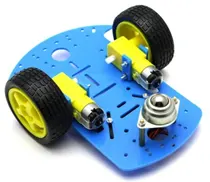
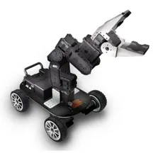
First of all, we are going to review the kinematic model of a Uniqlo type robot in these two images (fig 01) we can Observe two types of hemicycle robot configurations. The first we have two wheels with a rotating wheel or idler wheel and the second we have one with four wheels which has two motors. Each motor will drive two wheels through some type of mechanism, either by pulleys, chains, or another mechanism to make the model of any type of robot. In addition, we have also put you in orientation.
First one Second one
Fig 01: Uniqlo-type robots.
In the first place, we are going to draw the reference system in this case the x plane. Next, we are going to draw our robot and we are going to draw it in a different position than from the origin as in this case, our robot has been drawn in a position x1 and y1 in a position (fig:02).
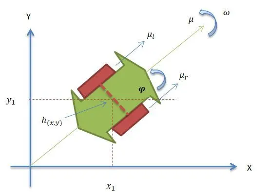
Fig(02): Geomatri diagram of robot kinematic.
As we can see here (fig:02) we have an orientation and what is the given kinematic model for the control actions entered. In this case, the linear speed of the left rim and the speed linear of the right rim we can find the position of our robot in our control point. It is our point of interest to which we need to know the position. That is, for example, we need to know the position at this point of the robot can be the center of mass or, we can also in this case our point of interest would be at the base of our manipulator. Then depending on the application our point of interest may change.
This time we are going to review the part that we had mentioned, that is, in the center of the robot. Our total system is going to have a linear speed that allows our robot to move forward and backward we have our angular velocity that allows the robot to rotate clockwise and in counter-clockwise
Now we are going to start with the mathematical part in this case we are going to review everything Using Geometry(fig:02).
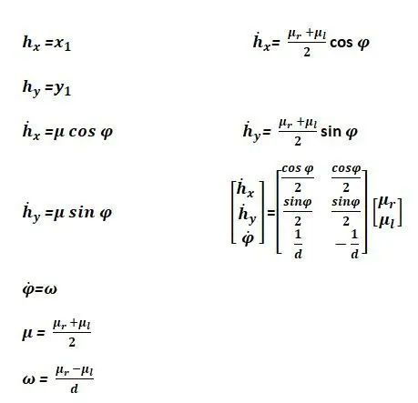
We are going to implement all of these equations in MATLAB for the observation of kinematic model simulation.
#Matlab code for 0 linear velocities of right and left wheel:
% Md Rubayat Alam Riad%


clc  % Clear Command Window
clear %Remove items from workspace, freeing up system memory
close all % Remove specified figure

ts=0.1; % sample time
t=0:ts:30; % vector time

ur=0*ones(1,length(t)); % linear velocity (right wheel)
ul=0*ones(1,length(t));% linear velocity (left wheel)


hx(1)=0;   % initial position (x axis) in m
hy(1)=0;   % initial position (y axis) in m
phi(1)=0;  % initial orientation in rad

d=0.5; % distance between wheels

for k=1:length(t)  % Loop simulation

     % Kinematic Model
    hxp(k)=((ur(k)+ul(k))/2)*cos(phi(k));
    hyp(k)=((ur(k)+ul(k))/2)*sin(phi(k));
    phip(k)=(ur(k)-ul(k))/d;

    %numerical integral (Euler Method)
    hx(k+1)=hx(k)+ts*hxp(k);
    hy(k+1)=hy(k)+ts*hyp(k);
    phi(k+1)=phi(k)+ts*phip(k);

end

scene=figure;  % new figure
tam=get(0,'ScreenSize');
set(scene,'position',[tam(1) tam(2) tam(3) tam(4)]); % position and size figure in the screen
axis equal; % Set axis aspect ratios
axis([-2 4 -2 2 -0.5 1]); % Set axis limits
view([135 35]);
grid on; % Display axes grid lines

MobileRobot; % Parameters of robot
M1=MobilePlot(hx(1),hy(1),phi(1)); % Plot robot in initial position hx,hy and phi orientation
hold on; % Retain current plot when adding new plot
M2=plot3(hx(1),hy(2),zeros(1),'r'); % plot trayectory.
xlabel('x(m)'); ylabel('y(m)'); zlabel('z(m)'); % Label axis
camlight right

step=10; % position step

for i=1:step:length(t) % Loop emulation
    delete (M1)
     M1=MobilePlot(hx(i),hy(i),phi(i)); hold on
     plot3(hx(1:i),hy(1:i),zeros(1,i),'b','LineWidth',2); % plot trayectory.
    pause(ts)
end
The functions we have used:
Function:01
function  Mobile_Graph=MobilePlot(dx,dy,angz)
global  Uniciclo;

% Matriz de rotación z

Rz=[ cos(angz) -sin(angz) 0; sin(angz) cos(angz) 0; 0 0 1];


%%%%%%%%%%%%%%%%%%%%%%%%%%%%%%%%%%%%%%%%%%%%
robotPatch = Rz* Uniciclo.platformVertices;
robotPatch(1,:)=robotPatch(1,:)+dx;
robotPatch(2,:)=robotPatch(2,:)+dy;

Mobile_Graph(1) = patch('Faces',Uniciclo.platformFaces,'Vertices',robotPatch','FaceColor',[0.3 0.75 0.93],'EdgeColor','none');

robotPatch = Rz* Uniciclo.platformfVertices;
robotPatch(1,:)=robotPatch(1,:)+dx;
robotPatch(2,:)=robotPatch(2,:)+dy;

Mobile_Graph(2) = patch('Faces',Uniciclo.platformfFaces,'Vertices',robotPatch','FaceColor','green','EdgeColor','none');


%%%%%%%%%%%%%%%%%%%%%%%%%%%%%%%%%%%%%%%%%%%%

robotPatch = Rz* Uniciclo.wheelVertices;
robotPatch(1,:)=robotPatch(1,:)+dx;
robotPatch(2,:)=robotPatch(2,:)+dy;

Mobile_Graph(3) = patch('Faces',Uniciclo.wheelFaces,'Vertices',robotPatch','FaceColor',[0.8 0.8 0.8],'EdgeColor','none');

robotPatch = Rz* Uniciclo.wheelBVertices;
robotPatch(1,:)=robotPatch(1,:)+dx;
robotPatch(2,:)=robotPatch(2,:)+dy;

Mobile_Graph(4) = patch('Faces',Uniciclo.wheelBFaces,'Vertices',robotPatch','FaceColor','black','EdgeColor','none');
Function:02
function  Mobile_Graph=MobilePlot(dx,dy,angz)
global  Uniciclo;

% Matriz de rotación z

Rz=[ cos(angz) -sin(angz) 0; sin(angz) cos(angz) 0; 0 0 1];


%%%%%%%%%%%%%%%%%%%%%%%%%%%%%%%%%%%%%%%%%%%%
robotPatch = Rz* Uniciclo.platformVertices;
robotPatch(1,:)=robotPatch(1,:)+dx;
robotPatch(2,:)=robotPatch(2,:)+dy;

Mobile_Graph(1) = patch('Faces',Uniciclo.platformFaces,'Vertices',robotPatch','FaceColor',[0.3 0.75 0.93],'EdgeColor','none');

robotPatch = Rz* Uniciclo.platformfVertices;
robotPatch(1,:)=robotPatch(1,:)+dx;
robotPatch(2,:)=robotPatch(2,:)+dy;

Mobile_Graph(2) = patch('Faces',Uniciclo.platformfFaces,'Vertices',robotPatch','FaceColor','green','EdgeColor','none');


%%%%%%%%%%%%%%%%%%%%%%%%%%%%%%%%%%%%%%%%%%%%

robotPatch = Rz* Uniciclo.wheelVertices;
robotPatch(1,:)=robotPatch(1,:)+dx;
robotPatch(2,:)=robotPatch(2,:)+dy;

Mobile_Graph(3) = patch('Faces',Uniciclo.wheelFaces,'Vertices',robotPatch','FaceColor',[0.8 0.8 0.8],'EdgeColor','none');

robotPatch = Rz* Uniciclo.wheelBVertices;
robotPatch(1,:)=robotPatch(1,:)+dx;
robotPatch(2,:)=robotPatch(2,:)+dy;

Mobile_Graph(4) = patch('Faces',Uniciclo.wheelBFaces,'Vertices',robotPatch','FaceColor','black','EdgeColor','none');
Simulation Results:
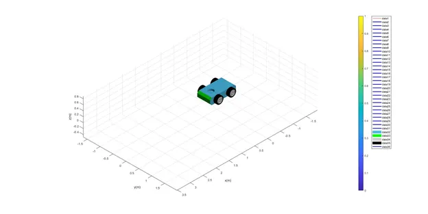
Fig 03: o linear velocity position of Robot.
#Simulation test of changing linear velocity(left & right wheel) in line no 8 & 9:

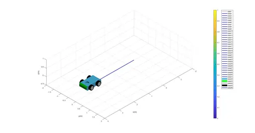
Fig 04: 0.1 linear velocity position of Robot.
# Matlab coding for circular movement:
clc  % Clear Command Window
clear %Remove items from workspace, freeing up system memory
close all % Remove specified figure

ts=0.1; % sample time
t=0:ts:20; % vector time

d=0.5; % distance between wheels
a=0.35; % distance a


ur=0.1*ones(1,length(t)); % linear velocity (right wheel)
ul=-0.1*ones(1,length(t)); % linear velocity (left wheel)

% initial center position of robot
x1(1)=0;   % initial position (x axis) in m/s
y1(1)=0;   % initial position (y axis) in rad/s
phi(1)=0;  % initial orientation in rad

% initial point control of robot
hx(1)=x1(1)+a*cos(phi(1));
hy(1)=y1(1)+a*sin(phi(1));


for k=1:length(t)  % Loop simulation

    % Kinematic Model
    hxp(k)=((ur(k)+ul(k))/2)*cos(phi(k))-a*((ur(k)-ul(k))/d)*sin(phi(k));
    hyp(k)=((ur(k)+ul(k))/2)*sin(phi(k))+a*((ur(k)-ul(k))/d)*cos(phi(k));
    phip(k)=(ur(k)-ul(k))/d;

    %numerical integral (Euler Method)
    hx(k+1)=hx(k)+ts*hxp(k);
    hy(k+1)=hy(k)+ts*hyp(k);
    phi(k+1)=phi(k)+ts*phip(k);

    %center position of robot
    x1(k+1)=hx(k+1)-a*cos(phi(k+1));
    y1(k+1)=hy(k+1)-a*sin(phi(k+1));

end

scene=figure;  % new figure
tam=get(0,'ScreenSize');
set(scene,'position',[tam(1) tam(2) tam(3) tam(4)]); % position and size figure in the screen

axis equal; % Set axis aspect ratios
axis([-4 4 -2 2 -0.1 1]); % Set axis limits
grid on; % Display axes grid lines

MobileRobot; % Parameters of robot
M1=MobilePlot(x1(1),y1(1),phi(1)); % Plot robot in initial position hx,hy and phi orientation
hold on; % Retain current plot when adding new plot
M2=plot(hx(1),hy(2),'r'); % plot trayectory.

xlabel('x(m)'); ylabel('y(m)'); zlabel('z(x)'); % Label axis
camlight('rigth');
step=10; % position step

for i=1:step:length(t) % Loop emulation

    delete (M1)
    M1=MobilePlot(x1(i),y1(i),phi(i)); hold on
     plot(hx(1:i),hy(1:i),'b','LineWidth',2); % plot trayectory.
    pause(ts)
end
Simulation results:
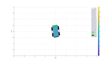
Fig 04: 2D view of circular movement.
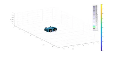
Fig 05: 3D view of circular movement.