Week 2 Air standard Cycle

Title: Air standard Cycle.

Objective: To write a python Code Program to Plot a P-V diagram for an Otto –cycle for given geometric volumetric parameters at a particular compression ratio and calculate the thermal efficiency of system as well.

Engine Design and Operating Parameters (Important Engine Characteristics):

Design Requirements:

• Good engine performance over entire operating range.
• Cost of fuel to be kept within limits.
• Low engine noise and pollution in this range.
• Low initial cost installation costs.
• Reliability and durability, maintenance requirements and how they affect engine cost etc.

Engine performance is defined by:

• Maximum power (or max. torque) available at each speed within useful range.
• Range of speed power over which engine operation satisfactory.

Some definition:

• Maximum rated power: Highest power engine is allowed to develop for short periods, also referred to as “Intermittent power rating”.
• Normal rated power: Highest power engine allowed developing in “continuous rating”.

Rated speed: Speed at which rated power is developed.

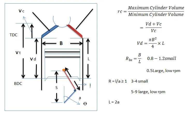
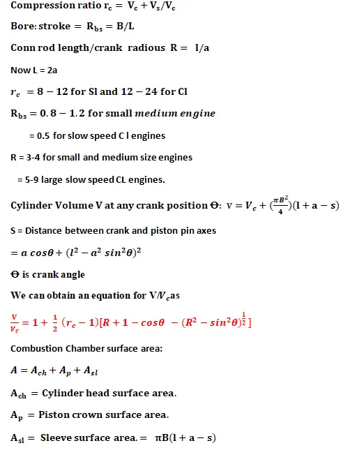
CYLINDER GEOMETRY

""""
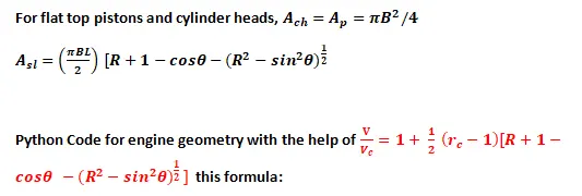
    Engine kinematics
"""
import math
import matplotlib.pyplot as plt 
#Geomatric parameters

bore = 0.10
stroke = 0.1
con_rod = 0.15
cr = 12
a = stroke/2
R = con_rod/a

#volume Parameters
V_s = math.pi*(1/4)*pow(bore,2)*stroke
V_c = V_s/(cr-1)

theta = math.radians(180)


term1 = 0.5*(cr-1)
term2 = R + 1 - math.cos(theta)
term3 = pow(R,2) - pow(math.sin(theta),2)
term3 = pow(term3, 0.5)

v = (1 + term1*(term2 - term3))*V_c

print(V_c+V_s)
print(v)

Result: 0.0008567979964335801

0.0008567979964335802

[Finished in 4.1s]

Note: Using the Python Code for engine geometry we have to solve Otto cycle problem.

OTTO CYCLE

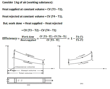
This cycle is so named as it was conceived by ‘Otto’. On this cycle, petrol, gas and many types of oil engines work. It is the standard of comparison for internal combustion engines.

Figs. (a) and (b) shows the theoretical p-V diagram and T-s diagrams of this cycle respectively.

1. The point 1 represents that cylinder is full of air with volume V1, pressure p1 and absolute temperature T1.
2. Line 1-2 represents the adiabatic compression of air due to which p1, V1 and T1 change to p2, V2 and T2, respectively.
3. Line 2-3 shows the supply of heat to the air at constant volume so that p2 and T2 change to p3 and T3 (V3 being the same as V2).
4. Line 3-4 represents the adiabatic expansion of the air. During expansion p3, V3 and T3 change to a final value of p4, V4 or V1 and T4, respectively.
5. Line 4-1 shows the rejection of heat by air at constant volume till original state (point 1) reaches.

Python Code for the Otto cycle simulator:

'''''
    otto cycle simulator 
'''

import math
import matplotlib.pyplot as plt 


def engine_kinematics(bore, stroke, con_rod, cr, start_crank, end_crank):
	""""
	    Engine kinematics
	"""
	#Geomatric parameters
	a = stroke/2
	R = con_rod/a

	#volume Parameters
	V_s = math.pi*(1/4)*pow(bore,2)*stroke
	V_c = V_s/(cr-1)

	sc = math.radians(start_crank)
	ec = math.radians(end_crank)
	
	num_values = 60

	dtheta = (ec-sc)/(num_values-1)

	v=[]

	for i in range(0, num_values):
		theta = sc + i*dtheta
		term1 = 0.5*(cr-1)
		term2 = R + 1 - math.cos(theta)
		term3 = pow(R,2) - pow(math.sin(theta),2)
		term3 = pow(term3, 0.5)

		v.append((1 + term1*(term2 - term3))*V_c)
		
	return v

# inputs
p1 = 101325
t1 = 500
gamma =1.4
t3 = 2300

# geomatric paramiter
bore = 0.1
stroke = 0.1
con_rod = 0.15
cr = 8

# Volume computation 
v_s = (math.pi/4)*pow(bore,2)*stroke
v_c = v_s/(cr-1)
v1 = v_c + v_s


#state point 2
v2 = v_c

#p2v2^gamma = p1v1^gamma
p2 = p1*pow(v1,gamma)/pow(v2,gamma)

#p2v2/t2 = p1v1/t1 , rhs = p1v1/t1, p2v2/t2 = rhs , t2 = p2v2/rhs 
rhs = p1*v1/t1
t2 = p2*v2/rhs
v_compression = engine_kinematics(bore, stroke, con_rod, cr, 180, 0)

constant = p1*pow(v1,gamma)

p_compression = []

for v in v_compression:
	p_compression.append(constant/pow(v, gamma))




# state point 3
v3 = v2 

#p3v3/t3 = p2v2/t2, rhs = p2v2/t2 , p3 = rhs*t3/v3

rhs = p2*v2/t2
p3 = rhs*t3/v3

v_expantion = engine_kinematics(bore, stroke, con_rod, cr, 0, 180)

constant = p3*pow(v3,gamma)

p_expantion = []

for v in v_expantion:
	p_expantion.append(constant/pow(v, gamma))
# state point 4
v4 = v1 

#p4*v4^gamma = p3v3^gamma

p4 = p3*pow(v3,gamma)/pow(v4,gamma)


# p4v4/t4 = rhs
t4 = p4*v4/rhs
#print(t4)

plt.plot([v2,v3,],[ p2,p3])
plt.plot(v_compression, p_compression)
plt.plot(v_expantion,p_expantion)
plt.plot([v4,v1,],[ p4,p1])
plt.show()

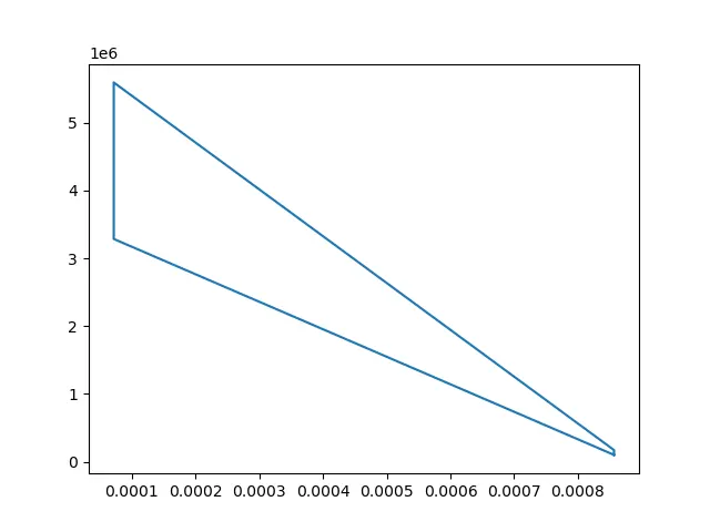
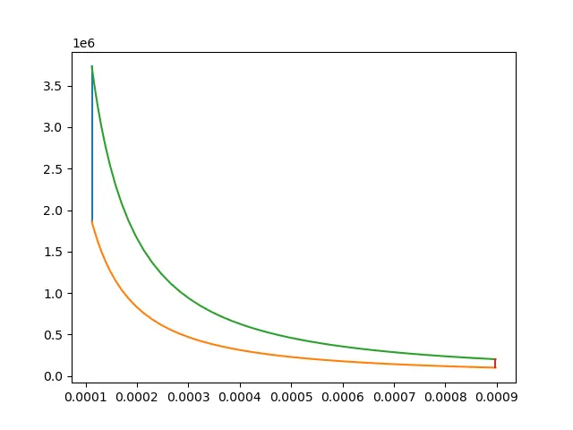
Output: Now the output of above is a follows:

Plots:

1) Using state variables:

P-v diagram for Otto cycle using volume tracing at cr = 08

2) Using volume traces:

P-v diagram for Otto cycle using volume tracing at cr = 08

Consolation:

Using this program as a template, for various combinations of geometric parameters- stroke and bore, connecting rod length etc. and volumetric parameters – clearance volume, swept volume etc... And a output showing ‘p –v’, a‘t-s’ diagramed thermal efficiency can be acquired which could save time and effort of the designers