Week 3 - Solving second order ODEs

Title: Simulation of the Transient Behaviour of a Simple pendulum by solving ODEs.

Introduction:

In Engineering, ODE is used to describe the transient behavior of a system. A simple example is a pendulum

The way the pendulum moves depends on Newtons second law. When this law is written down, we get a second order Ordinary Differential Equation that describes the position of the "ball" w.r.t time.

Similarly, there are hundreds of ODEs that describe key phenomena and if you have the ability to solve these equations then you will be able to simulate any of these systems.

Your objective is to write a program that solves the following ODE. This ODE represents the equation of motion of a simple pendulum with damping

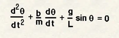
In the above equation,

g = gravity in m/s2,

L = length of the pendulum in m,

m = mass of the ball in kg,

b=damping coefficient.

Write a program in Matlab\Octave that will simulate the pendulum motion, just like the one shown in the start of this challenge.

use,

L=1 metre,

m=1 kg,

b=0.05.

g=9.81 m/s2.

Simulate the motion between 0-20 sec, for angular displacement=0,angular velocity=3 rad/sec at time t=0.

Solution of ODE:

Theta = theta1

d theta / dt = dtheta/dt = theta2

d^2theta/ dt^2 = d^2theta1/dt^2=dtheta2/dt

By this,

dtheta1/dt = theta2

dtheta2/dt=-|(b/m)theta2 – (g/l)sin(theta)

Solution for theta:

d/dt[theta1,theta2]=[theta2,-|(b/m)heta2-(g/l)sin(theta)]

Program for cooling a function:

function[dtheta_dt] = ODE_FUNC(t,theta,b,g,l,m)
theta1= theta(1);
theta2=theta(2);
dtheta1_dt=theta2;
dtheta2_dt=-(b/m)*theta2-(g/l)*sin(theta1);
dtheta_dt=[dtheta1_dt;dtheta2_dt];
end

Code explenation:

In the above program, we are using the function command for giving the inputs and solving the second-order ODEs equation.

And we are solving the solution vector dtheta1_dt and determining it in the main program.

Program For solving ODE:

clear all
close all
clc
% input value
b=0.05;
g=9.81;
l=1;
m=0.1;


%include condition
theta0=[0;4];

%time points

time=linspace(0,20,500);

%solving ode

[a,b]=ode45(@(t,theta)ODE_FUNC(t,theta,b,g,l,m),time,theta0)
%pliting

figure(1)
plot(a,[b(:,1) b(:,2)])
    
xlabel('Time in sec')
ylabel('Angular Displacement & Angular Velocity(rad/sec)')
legend('Angular Displacement','Angular Velocity(rad/sec)')
axis([0 23 -2 2])
hold on

%Simulation of pendulum
theta = b(:,1);
c=1;
for i = 1:length(theta)
theta1 = theta(i);

x0=0;
y0=0;

x1=l*sin(theta1);
y1=-l*cos(theta1);

figure(2)

plot([-1.4 1.4],[0 0],'linewidth',5,'color','g')
hold on
plot([x0 x1],[y0 y1], 'color','b','linewidth',3);
hold on

plot(x1,y1,'O','markers',30,'color','r','markerfacecolor','r');

hold off
axis([-1.5 1.5 -1.5 0.5])
pause(0.003)
M(c)=getframe(gcf);
c=c+1;
end
movie(M)
videofile=VideoWrite('pendulum.avi','uncompressed AVI');
open(videofile)
writeVideo(videofile,M)
close(Videofile)

Output for figure 1:

.

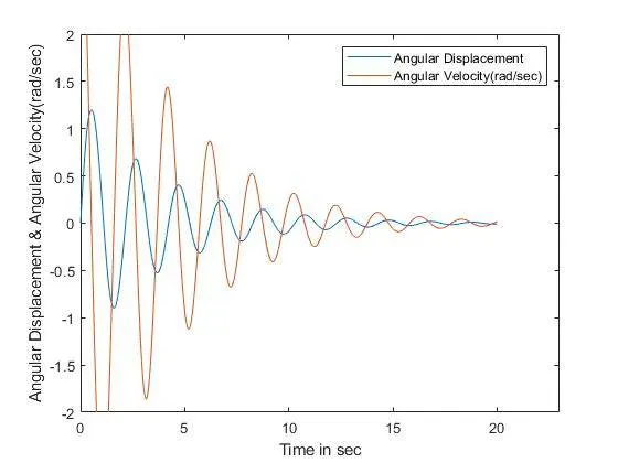
Output for figure2:

https://youtu.be/ggMoZi4-ceg?t=3

Simple Pendulum Animation