Exhaust Port Challenge

Aim:

1. Give a brief description of why and where a CHT analysis is used.
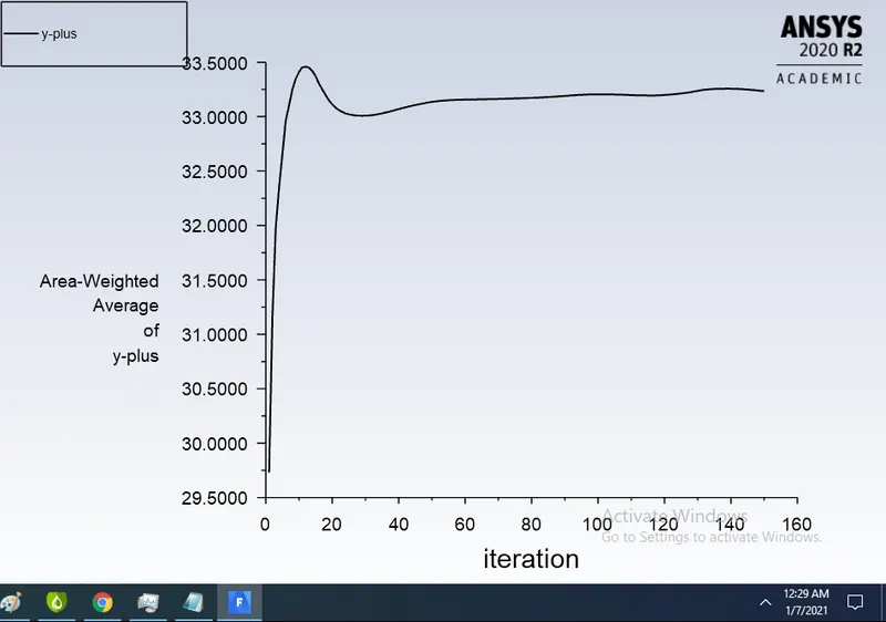
2. Maintain the y+ value according to the turbulence model and justify the results.
3. Calculate the wall/surface heat transfer coefficient on the internal solid surface & show the velocity & temperature contours in appropriate areas.
4. How would you verify if the HTC predictions from the simulations are right? On what factors does the accuracy of the prediction depend on?

Conjugate Heat Transfer (CHT)

1.The Conjugate Heat Transfer (CHT) analysis allows for the simulation of heat transfer between solid and fluid domains by exchanging thermal energy at the interfaces between them.

2. The CHT approach therefore has benefits for those applications where heat transfer is either non-uniform or difficult to calculate empirically

3.conduction through solids, free and forced convection in the gases/fluids and thermal radiation.

4. Examples of CHT are conduction through solids, free and forced convection in the gases/fluids and thermal radiation.simulation of heat exchangers, cooling of electronic equipment, and general-purpose cooling and heating systems.

5.The CHT approach has an advantage overFE thermal analysis in that wall heat transfer coefficients and their local variations on surfaces are directly calculated within the model rather than based on simplified empirical calculations.

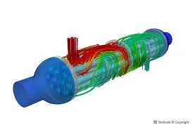
Applications:

1. Fuel rods in nuclear reactor, sheel and tube heatexchanger, aerospace,Food processing,medical applications and in metirology departments

Y+ value:

1. Y+ plus value for k-epsilon and k-omega are mainted as follows

2. For k-omega Range of Y+ is between(1m<y+<5m)

3.For k-epsilon Range of Y+ is between (30m<Y+<300m)

4. in exhaust port problem y+values for k-omega is taken as 5m and for k-epsilon taken as 75m

Procedure:

Geometry:

1. Insert solid exhaust port into space cliam.

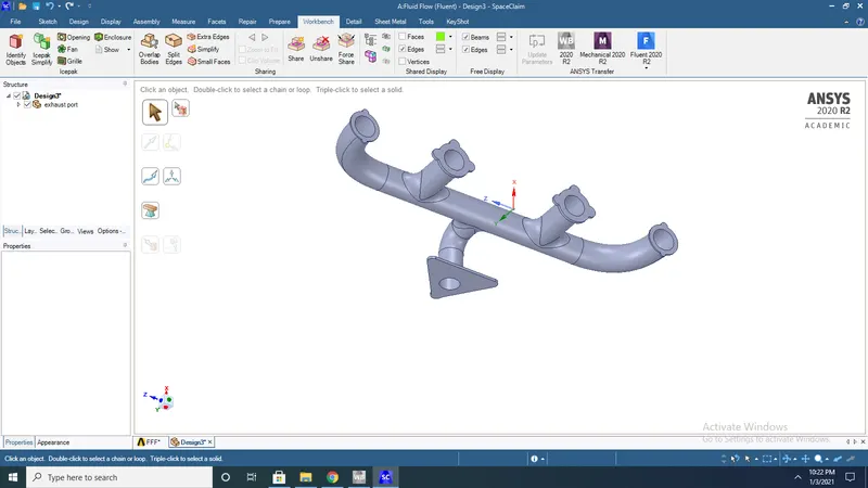
2. Remove extra edges of exhaust port for proper volume extraction.

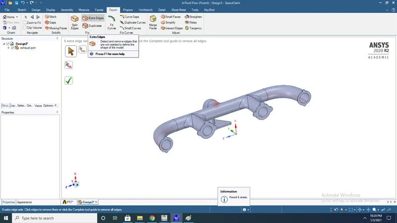
3. areas of extra edges(6) are fixed and solved

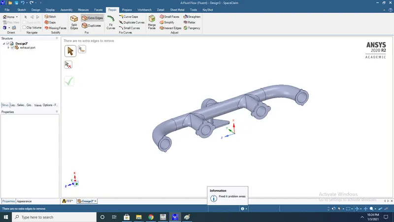
4. use volume extraction for inlet and outlet ports and name it as fluid volume

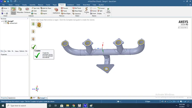
5. volume extraction of ports are done successfully

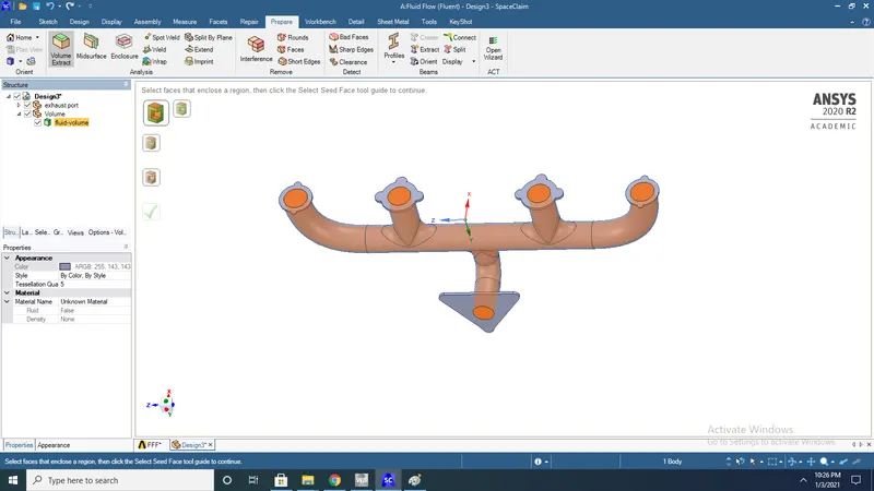
6. Enable share topology for geometry to get conformal mesh

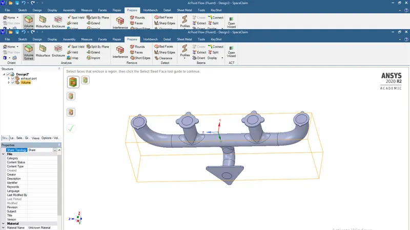
7.next create finalgeometry by selecting both volumes solid and fluid

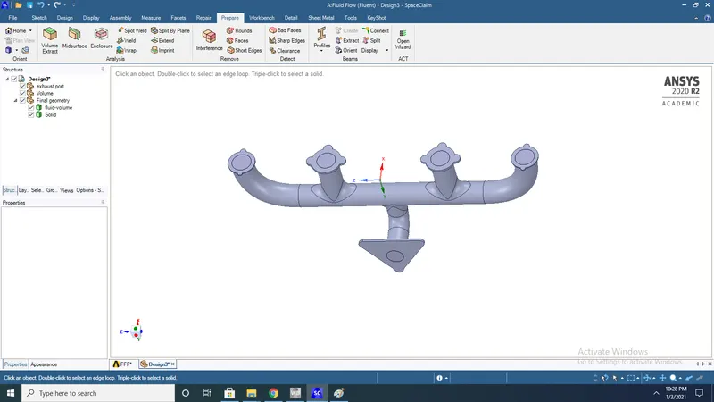
8.Delete empty components of geometry

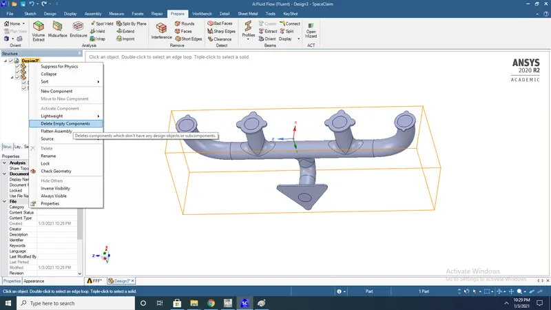
9.click share to avoid overlapping of edges,faces and volumes

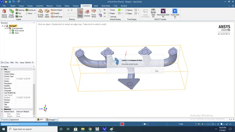
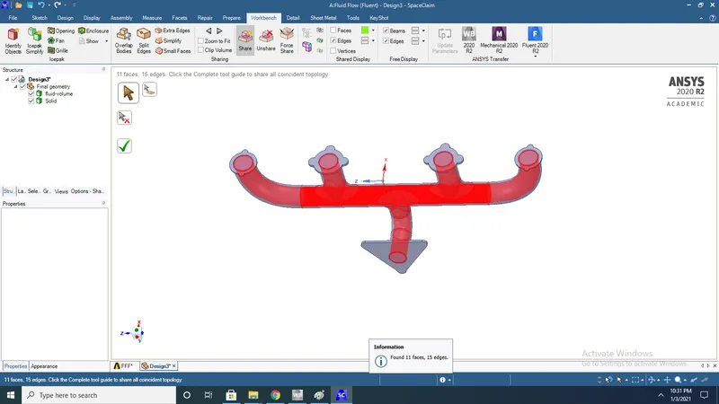
10.it shares 11 faces and 15 edges

9.

11. Pink circles shows areas of sharing in exhaust port

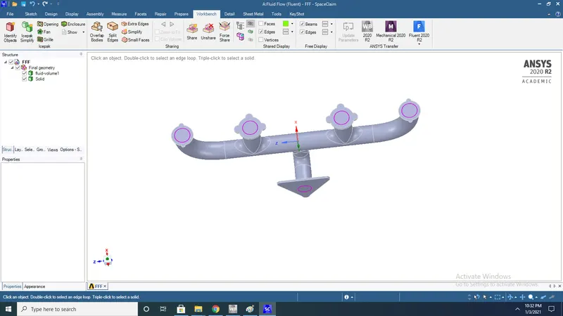
Meshing:

Named selections:

1.Inlet (4 edges)

2.outlet (1edge)

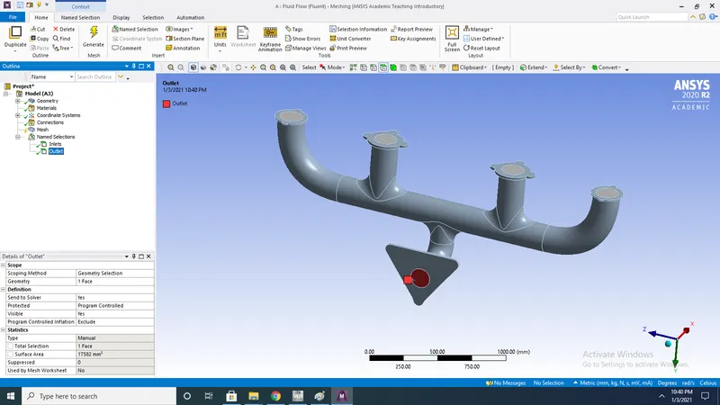
3.Outer wall convection(11 faces)

base linemesh:

4. Click generate mesh and itshows no of elements 137861

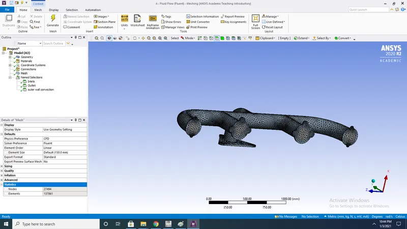
5. Quality of mesh

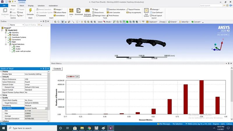
Refinment:

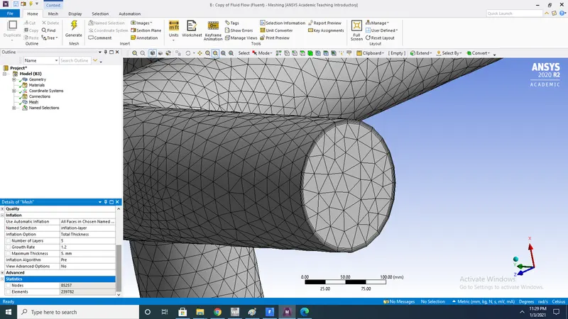
6. inorder to improve no of cells and quality you need to refine mesh by using option inflation max layers=5

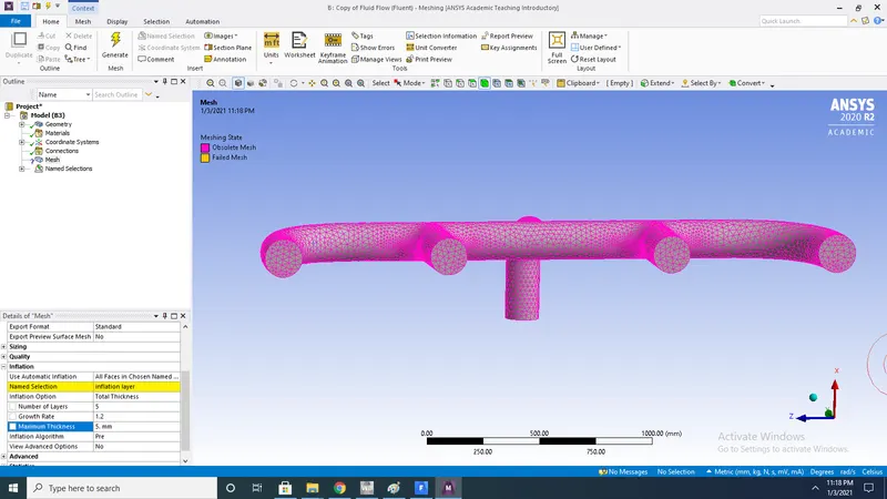
7.Magnified view shows 5 layers of inflation on inlet ports

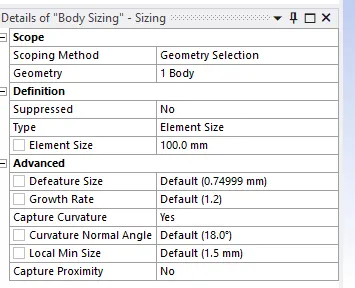
8 Body sizing on solid element around inlet ports to increase no of cells.

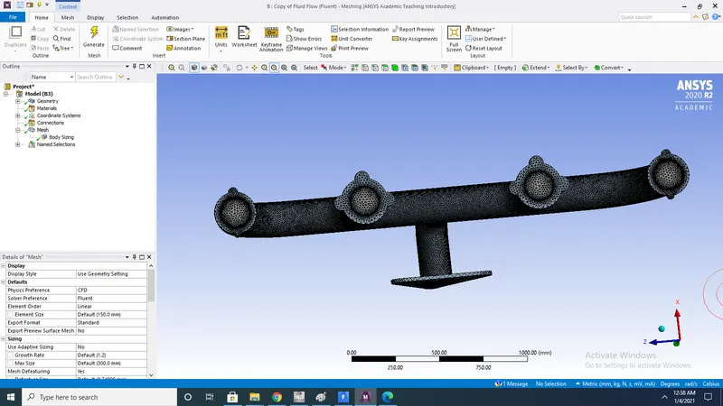
9.View shows body mesh of the inlet ports.

9. Finally refinment view of Exhaust port is shown along with statstics

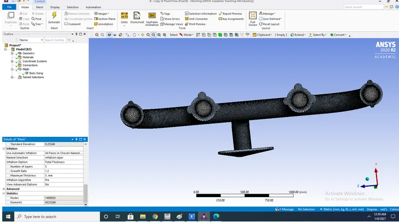
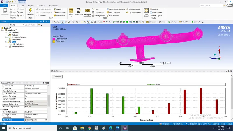
10.After refinment there is phenominal growth of elements, No of elements=4523266

11.Element Quality

Setup:

1)General

Type: Pressure-based

Time: steady

Velocity formulation: Absolute

2D Space : Planar

2)Models:

Viscous: Turbulent : K-epsilon,K-omega

3)Materials:

Fluid= Air

Solid= Aluminium

4)Cell zone conditions: Fluid

5)Boundary conditions:

Inlet:

Velocity=5m/s

Temperature=700K

Outer wall convection:

Heat transfer coefficent=20 W/m^2-k

Adiabatic wall:

Heat flux=zero

Intialization:

Hybrid intialization

Results:

Base line mesh:

K-omega:

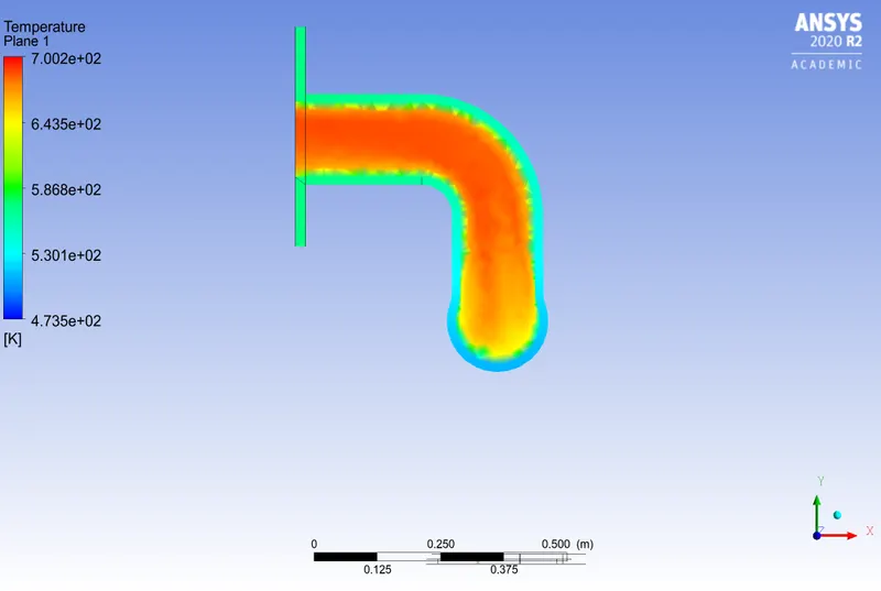
Temperature contour:

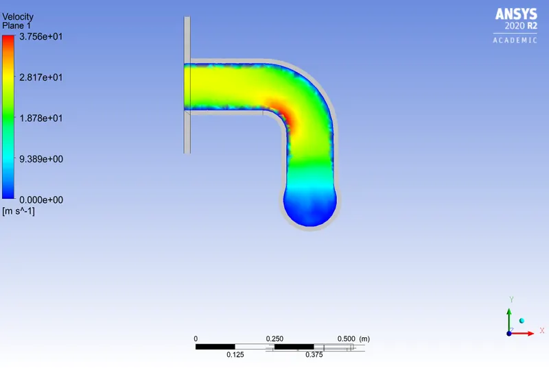
Velocity contour:

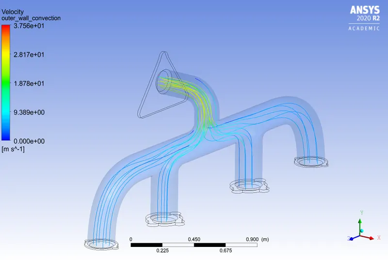
Velocity stream contour:

Wall heat transfer coefficent:

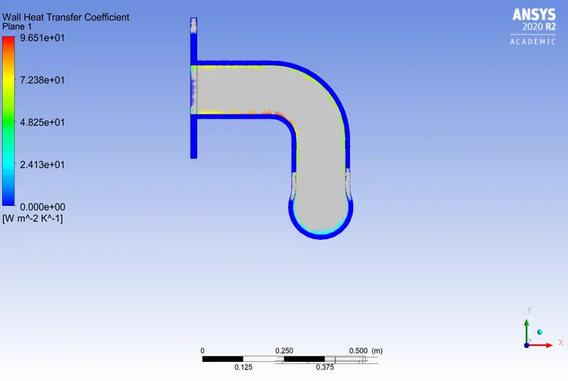
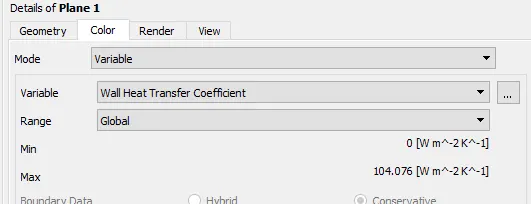
Value of heat transfer coefficent:

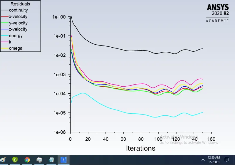
Residuals:

Y plus:

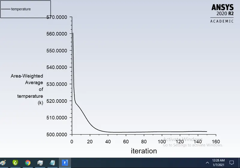
Area wegihted average of temperature:

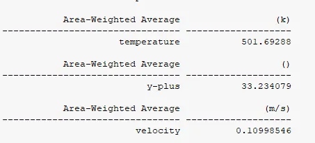
Values:

Base line mesh:

K-epsilon:

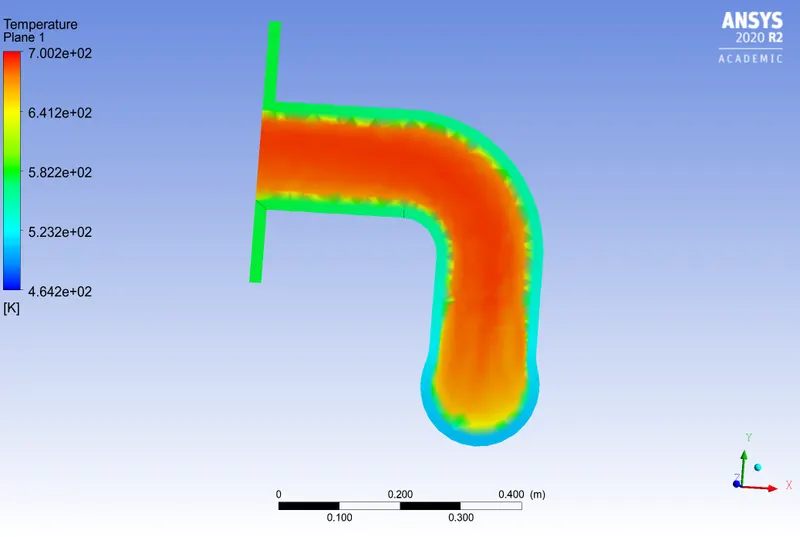
Temperature contour:

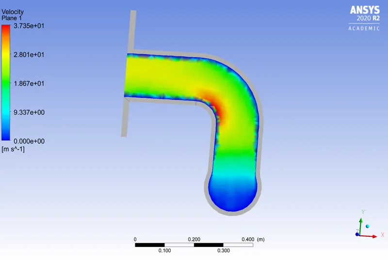
Velocity contour:

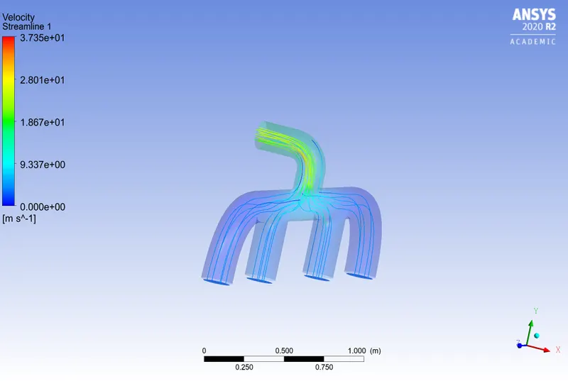
Velocity streams:

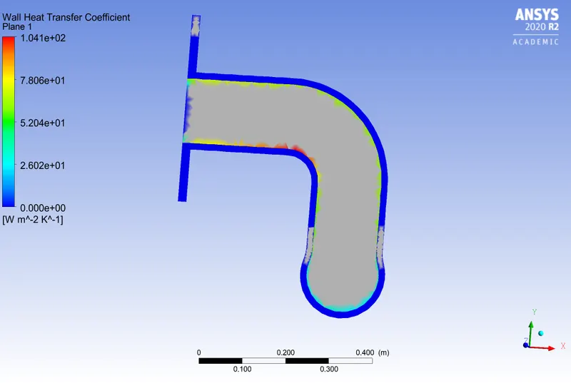
Wall heat transfer coefficent:

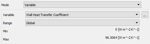
value of wall heat transfer coefficent:

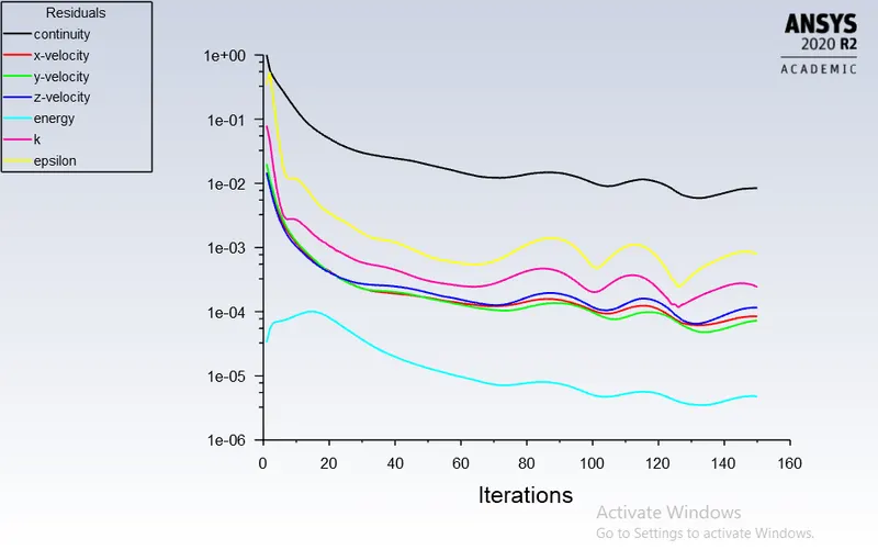
Residuals:

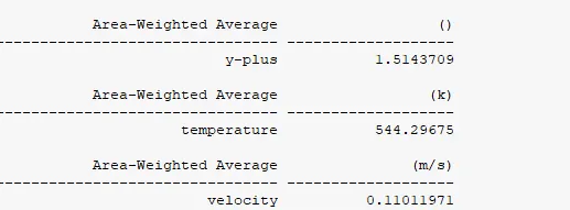
Y-plus:

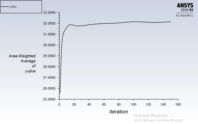
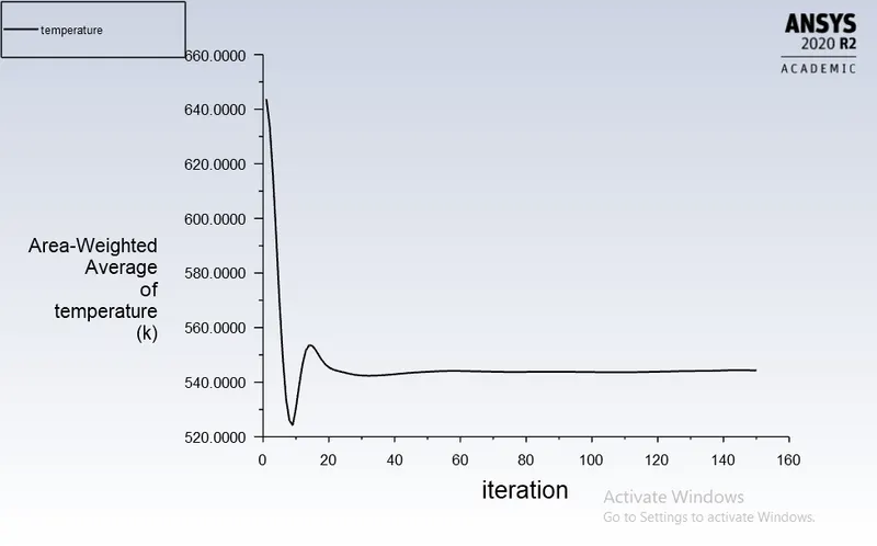
Area weighted average:

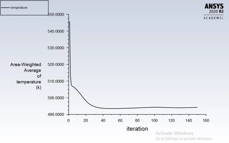
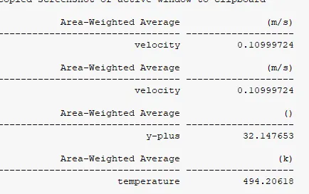
Values:

Refined mesh with inflation:

S.No	Turbulence model	Y(mm)	Y+(mm)	No of inflation layers
1	K-omega	0.3	5	5
2	K-epsilon	5	75	5

K-Omega(After refinement):

Temperature contour

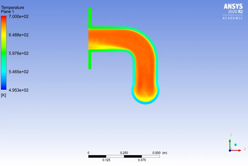
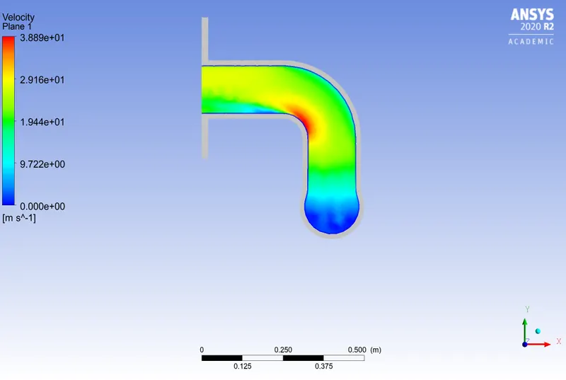
Velocity contour:

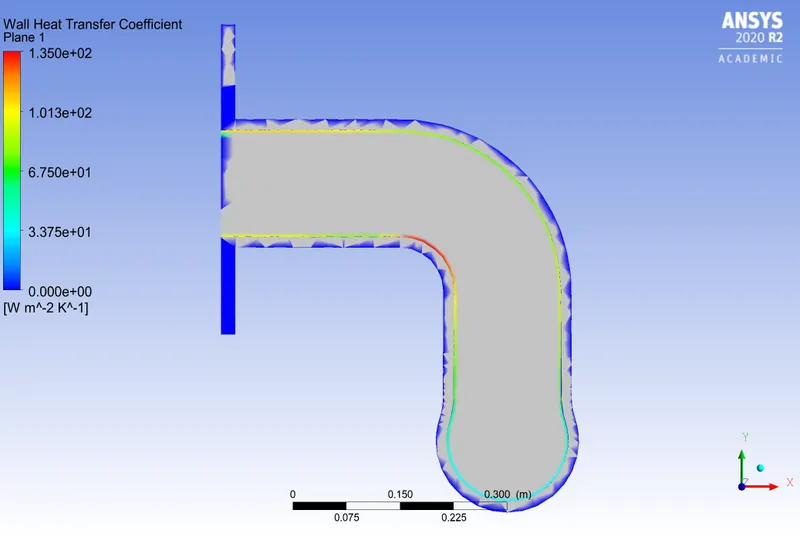
Heat transfer coefficent:

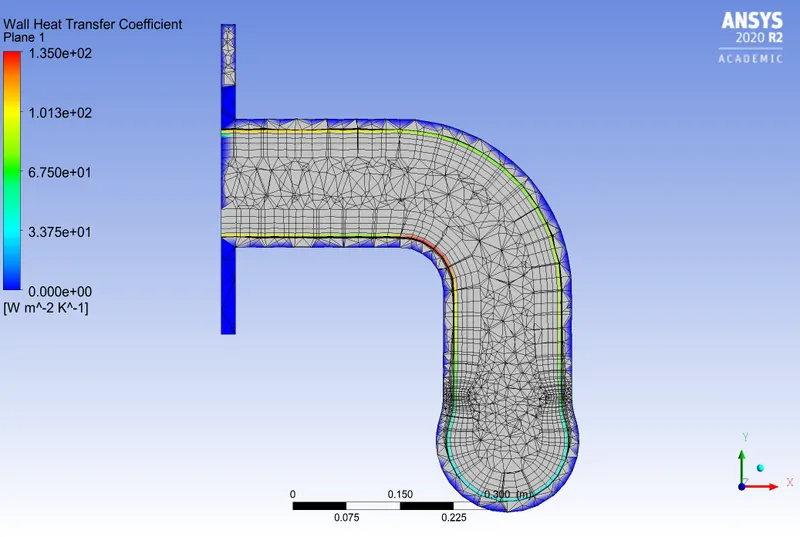
Heat transfer coefficent with mesh:

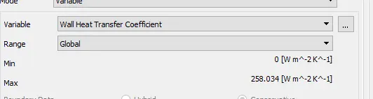
Values of heat transfer coefficent:

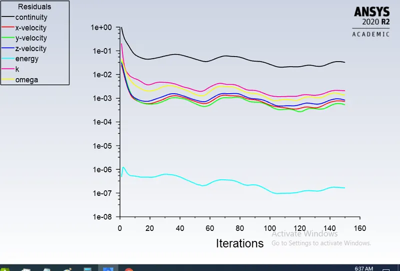
Residuals:

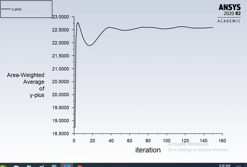
Y-Plus:

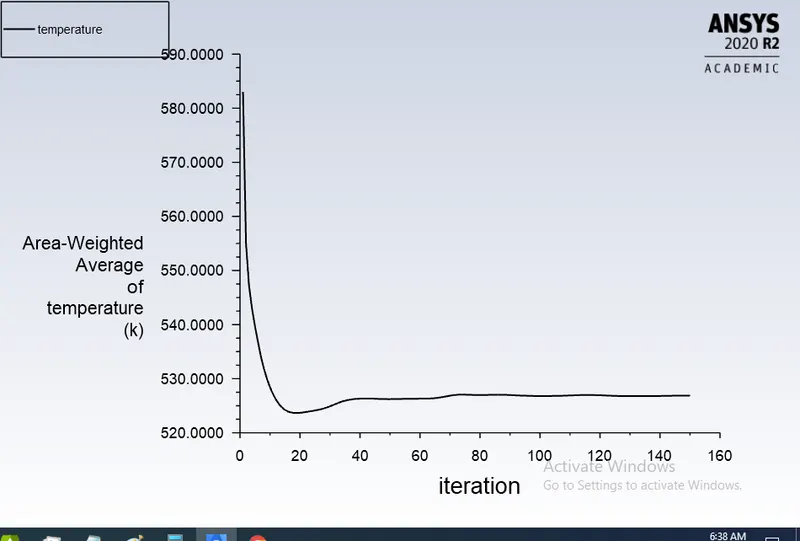
Average weighted temperatutre:

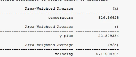
Values:

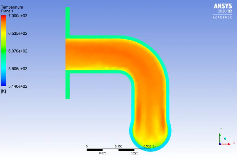
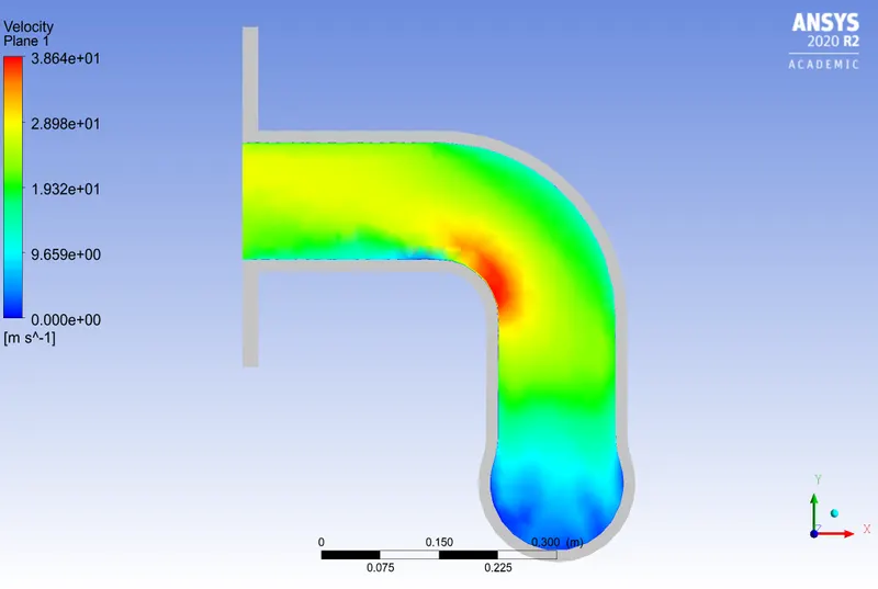
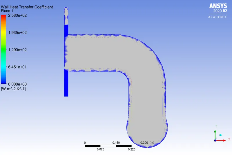
K-Epsilon(After refinement):

Temperature contour:

Velocity contour:

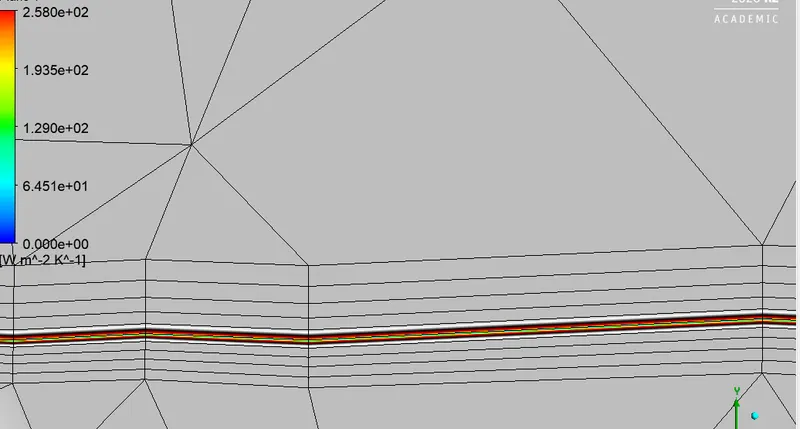
Heat transfer coefficent:

Heat transfer coefficent with mesh:

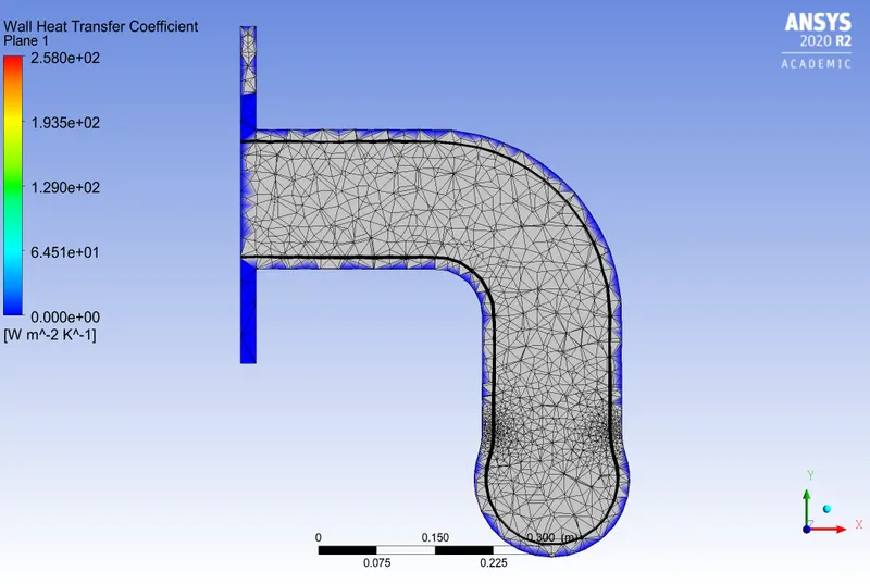
Showing inlation layers(Heat transfer coefficent):

Values of heat transfer coefficient:

Residuals:

Y-plus:

Area weighted average:

Values:

Comparision of results:

	K-omega (Base line mesh)	K-omega(After refinement)	K-epsilon(Base line mesh)	K-epsilon (After refinement)
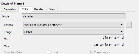
Heat transfer coefficent	104.076	258.034	96.5064	135.004
Y plus value	NN	75m	NN	5m
Y value	NN	5mm	NN	0.3mm

Correct turbulence model:

1.k-omega model of turbulence is capable of solving turbulence parameters very close to boundary or wall region. you have to have very fine meshing near to wall, so that Y+ value should be as small as possible.

2. k- epsilon provides standard results well far from the boundaries (wall) The k-ε model is more suitable when you are studying free-shear layers and wake region

3.From above results for conjugate heat transfer k-omega turbulence model gives higher heat transfer coefficent compared to k-epsilon model

Oservation:

1. Compared to base line mesh heat transfer coefficent is more in refinement mesh in both cases

2. which means better Y Plus value gives better refinement and results

3. Y plus plays important role in meshing and different turbulence models have different Y plus values.

Justification of Htc predications:

1.in free convection Nu=f(gr,pr)

2. in forced convectionNu=f(re,pr)

where Re=Reynolds number

gr=Grashoff number

pr= Prandtl number

similarly there are correlations for fluid flow in convection

Nu=C(Re^a*pr^b)

Nu=H*l/K

Where H= overall heat transfer coefficent

Lc= charcterstic length

k=thermal conductivity of pipe

(H*Lc)/K = C*(re^a * pr^b)

Where a,b,c are experimental values not known if we know them

we can compare with numerical solution values of heat transfer coefficent with experimental values of different turbulent models (k-epsilon,k-omega) to know right or wrong.