Conjugate Heat Transfer analysis on Exhaust port

Problem Definition

1. Why and where a CHT analysis is used.

2. We have to maintain the y+ value according to the turbulence model and justify the results.

3. Calculate the wall/surface heat transfer coefficient on the internal solid surface & show the velocity & temperature contours in appropriate areas.

4. How would you verify if the HTC predictions from the simulations are right? On what factors does the accuracy of the prediction depend on?

Introduction

Conjugate Heat Transfer (CHT)

The Conjugate Heat Transfer (CHT) analysis allows for the simulation of heat transfer between solid and fluid domains by exchanging thermal energy at the interfaces between them. In CHT we focus on conjugating the boundary condition at the fluid-solid interface through coupled heat transfer analysis. This coupled field is termed as Conjugate Heat Transfer (CHT).

Conjugate Heat Transfer (CHT) solver is used to understand the interface properties and flow properties due to change in the wall heating rates.

It is also useful to examine the heat penetration of solid in various wall materials with different time scales. CHT can also be used where the solution domain consists of more than one sub-domains in which heat transfer governed by different differential equations.

This model describes the heat transfer between a body and a fluid flowing over or inside it as a result of the interaction of two objects.

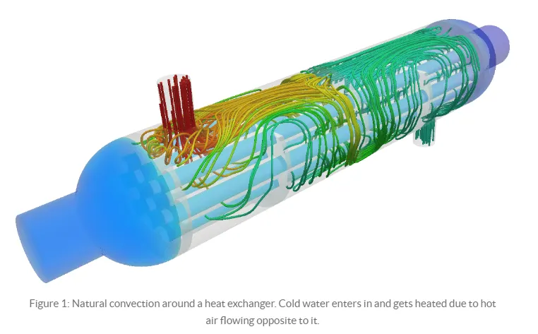
CHT studies are focused to understand the limit of applicability of the assumptions which are considered to recover the experimental data. It is also considered as a tool for simultaneous prediction of wall heat flux and temperature.

Conjugate heat transfer problems can be solved by either analytical methods or by numerical methods. The analytical CHT studies require a thorough understanding of the given heat transfer problem and involve complex mathematics. Such studies involve a lot of simplifications based on certain valid assumptions. Hence the correctness of the solution depends largely on the validity of assumptions made.

On the other hand, numerical CHT solution methods are relatively simpler if the numerical methods to be followed are clear. Moreover, a correctly implemented numerical CHT solver is not just limited to one CHT problem. Hence the same CHT algorithm can be applied to several CHT problems with minimum efforts in terms of solution domain modifications.

Application of CHT Analysis

CHT analysis is used in various applications to understand the heat transfer between two domains (solid and water or for more than two sub-domain). Some example:-

1. Heat transfer analysis in the cooled turbine blade Wang.

2. Measurement of the heat transfer coefficient in a Channel with Pin Fins.

3. Analysis of a Thermocouple Sensor in a Low-Temperature Nitrogen Gas Ambient.

4. Analysis of Natural Convection and Radiation Heat Transfer from Various Shaped Thin Fin-Arrays Placed on a Horizontal Plate.

5. Conjugate heat transfer and coupled field analysis is aerospace engineering.

6. Conjugate-Heat-Transfer ImmersedBoundary Method for Turbine Cooling.

7. Thermal Treatment of Materials.

Y+

The y+ value is a non-dimensional term that can be used to understand how coarse or fine our grid is.

Y+ value depends upon the first element. So to get the Y+ value small we need to make our first element very small and to get the Y+ value large we are gonna need the first element to be large. So in this challenge, we are going to use the inflation layer. We are going

where

y = distance from the wall

`u_t` = frictional velocity

`nu` = kinematic viscosity

We decide what turbulence model we need to choose on the basis of our Y+ value. If the Y+ value is less than 5 it is good to choose k-`omega` model but if the Y+ value is more than 30 we have to use k-`epsilon` model.

So in this challenge, we are going to use the inflation layer. We are going to use k-`omega` model so we have to keep the Y+ value to be less than 5. So keep that in mind we are going to give the first layer to be in that range so that the Y+ value does not go beyond the 5.

Case Setup

Case-1

Coarse Mesh

1. First we are going to open the workbench and going to click on the Fluid Flow(Fluent). It is going to open the module in the Project Schematic.

2. Now we are going to click on the geometry. It will take you to the spaceClaim. Here we are going to open the existing design. So now we can see the original design. On which we are going to do our simulation.

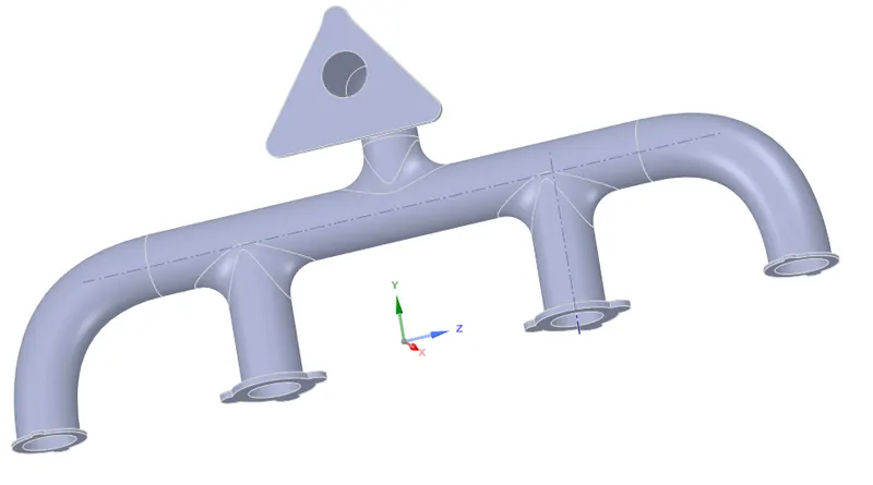
3. If there are any extra edges we need to remove them. In order to do that we will go to the workbench select the extra edge option and we are going to delete them one by one.

4. Now we are going to extract the fluid body. So to that, first we are going to create a new component after that we have to go to the Prepare option and we have to select the volume extract option. We are going to give that body name fluid and for the outer body, we are going to give that body name to be solid.

5. We want the flow of information in between both body so we are going to select the share option in the workbench.

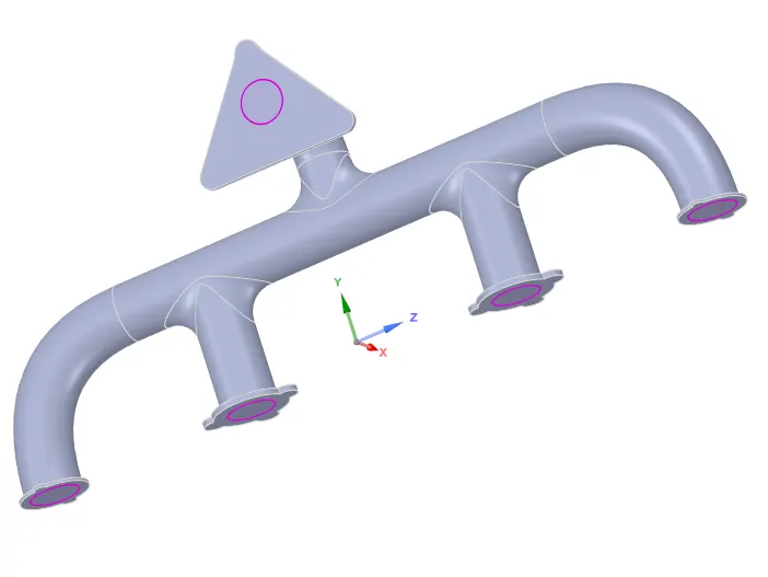
6. Now we are going to open the mesh and we are going to create the mesh with 50 mm element size.

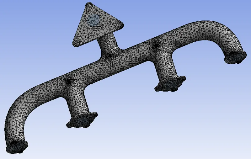
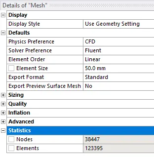
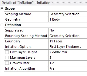
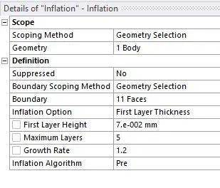
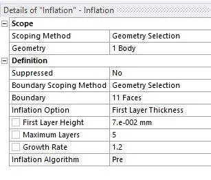
We are going to choose the model to be k-`omega` and for that Y+ value should be less than 5 so we are going to add inflation layers in the mesh. So for that, we are going to give the inflation layer on the fluid with first layer thickness to be 0.07 mm with a 20% growth rate and we are going to generate the mesh.

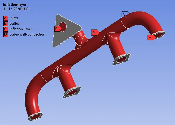
We are going to naming the body parts inlet, outlet, inflation layer and outer-wall-convection.

7. Now we are going to update the mesh. Now we are going to Setup the case. Here we are going to take the model to be turbulent k-`omega` SST model.

8. In the Fluent we will go to Physics. Here we choose the type of solver, we have taken the pressure-based type solver. The Mach number value is less than 0.33 that's why we are using pressure-based solver.

9. Now we have to choose the velocity formulation, we have taken absolute velocity formulation. Now we are going to choose the time, we are using a steady time. We want to calculate the heat transfer coefficient so we are going to consider the energy equation also.

10. Now we are going to give the initial boundary condition. So at the inlet, we are going to give 5 m/s inlet velocity and temperature to be 700k and at the outlet, we are going to give the pressure to be zero (static pressure).

We want the flow of information in between solid and fluid body so we are going to choose thermal conditions for the inflation layer to be coupled.

Now we are going to give the boundary condition to the outer-wall-convection. We are going to choose a thermal condition to be convection because we want the heat transfer between the fluid and solid. We are going to give the heat transfer coefficient value to be 20 `wm^-2k^-1`.

We are going to use the default materials. So we are using air to be the fluid material and aluminum to be solid material.

11. Now we are going to click on the solution. Here we are going to create the definitions.

12. Now we are going to initialize the solution, we are going to use the standard initialization and we are going to create the pressure and velocity contour.

13. Now we are going to simulate the result and we will get the plots and results.

Results

Residual

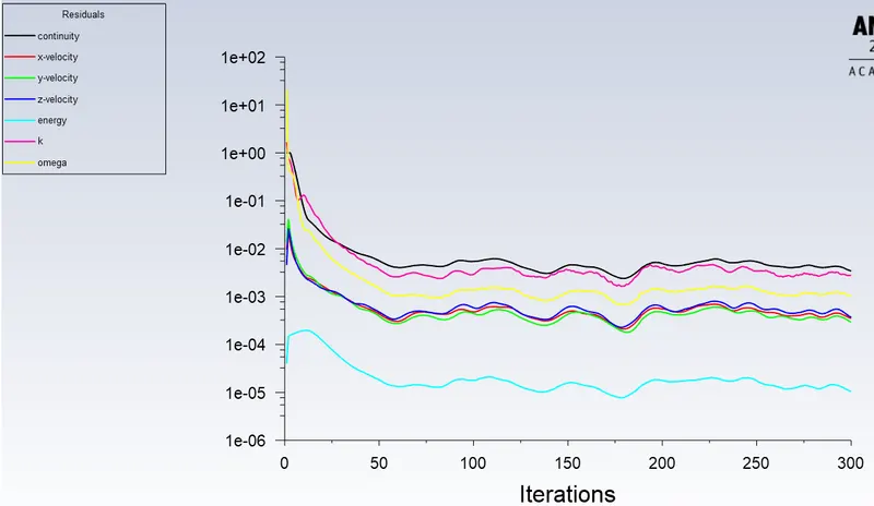
From the graph, we can see that we got the converged result. Because after some time it is repeating the same pattern.

Y+

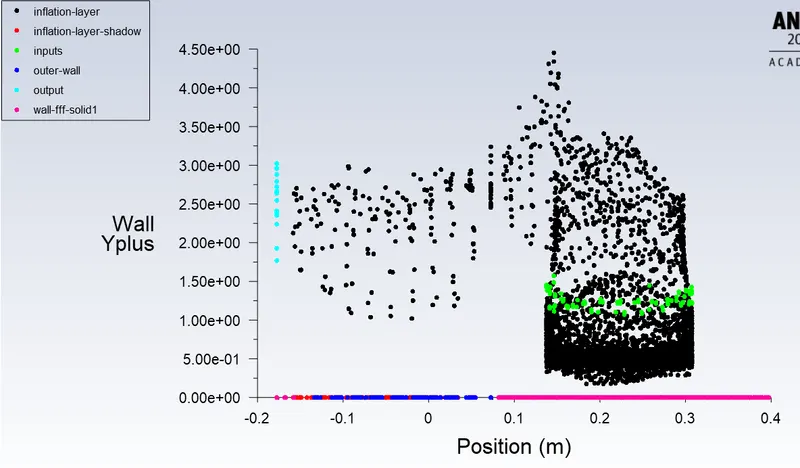
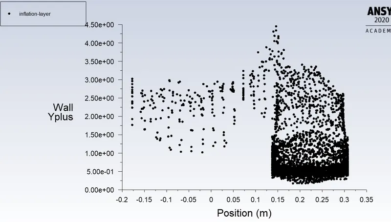
For the k-`omega` model Y+ value should be less than 5 and I'm getting Y+ value less than 5. So I can say that I have taken the right turbulence model. This will happen in every case.

Temperature at the Inflation Layer

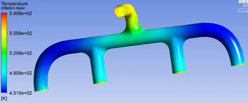
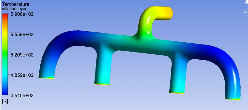
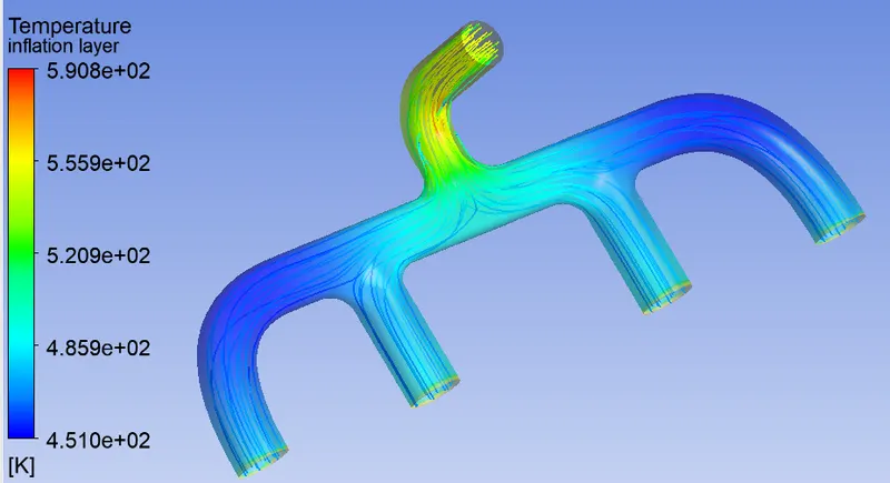
In the above picture, we can see the temperature distribution in the inflation layer. We are getting the maximum temperature at the outlet of the exhaust body. The maximum temperature we got is 590.8 k and the range of the temperature is 451 to 590.8 k.

Heat Transfer Coefficient at the Inflation Layer

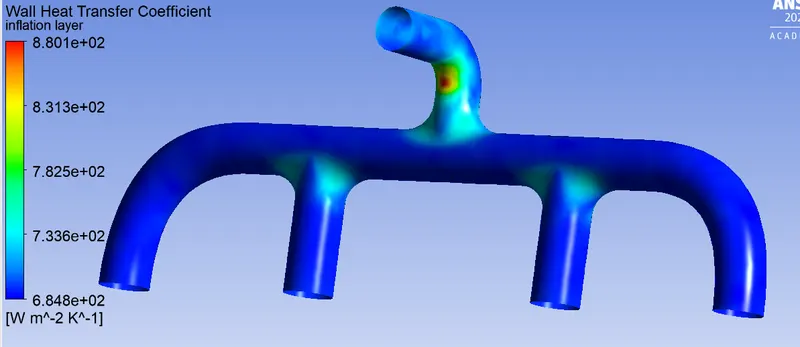
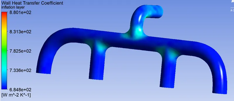
In the above picture we can see the heat transfer coefficient distribution in the inflation layer. The inflation layer is the surface of the internal solid surface in this case which is air. The maximum heat transfer coefficient value we got is 880.1 `Wm^-2K^-1`. The range of the heat transfer coefficient is 684.8 to 880.1 `Wm^-2K^-1`.

We can see from the above plots that at the bend near the outlet, velocity increases because of that there is an increase of the heat transfer coefficient. We got the maximum heat transfer coefficient there.

Velocity Streamlines

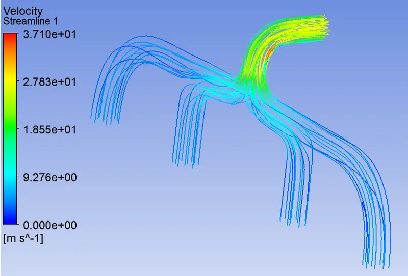
In the above picture we can see that the velocity distribution in the exhaust port. We can see that air is going from inlet to outlet and changing at different points in the port. The maximum velocity we got is 37.1 m/s and the range of the temperature is 0 to 37.1 m/s.

Velocity Streamline with Temperature at Inflation Layer

Temperatue at outlet plane

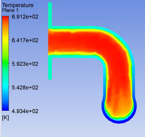
In the above picture, we can see the temperature distribution at the outlet of the exhaust port. The maximum temperature we got is 691.2 k and the range of the temperature is 493.4 to 691.2 k.

Velocity at outlet plane

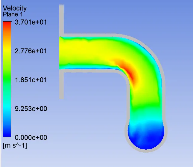
In the above picture, we can see the velocity distribution at the outlet of the exhaust port. The maximum velocity we got is 37.01 m/s and the range of the temperature is 0 to 37.01 m/s.

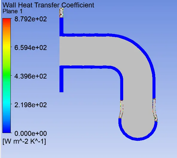
Wall Heat Transfer Coefficient outlet plane

Temperature at the outer wall

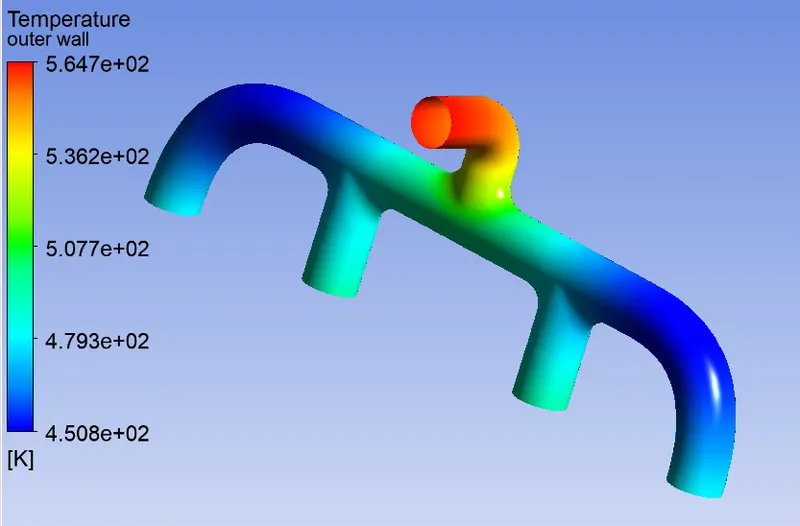
We can see from the above picture that the temperature in the outlet is high on the outer wall.

Case-2

Mesh

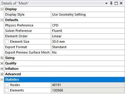
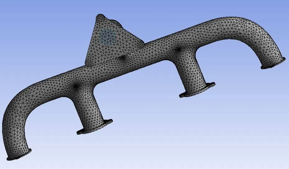
Heat Transfer Coefficient at the Inflation Layer

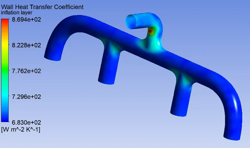
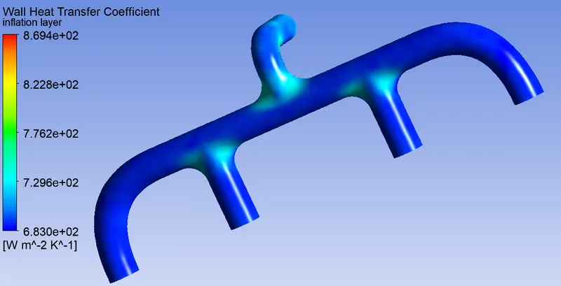
In the above picture we can see the heat transfer coefficient distribution in the inflation layer. The inflation layer is the surface of the internal solid surface in this case which is air. The maximum heat transfer coefficient value we got is 869.4 `Wm^-2K^-1`. The range of the heat transfer coefficient is 683.0 to 869.4 `Wm^-2K^-1`.

We can see from the above plots that at the bend near the outlet, velocity increases because of that there is an increase of the heat transfer coefficient. We got the maximum heat transfer coefficient there.

Temperature at the Inflation Layer

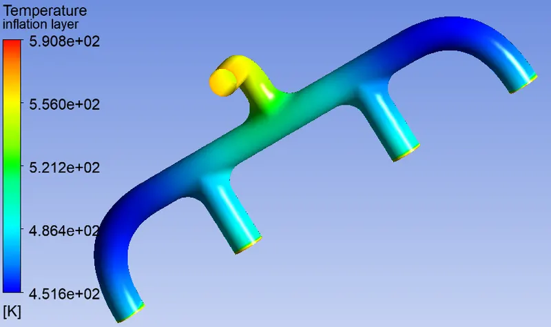
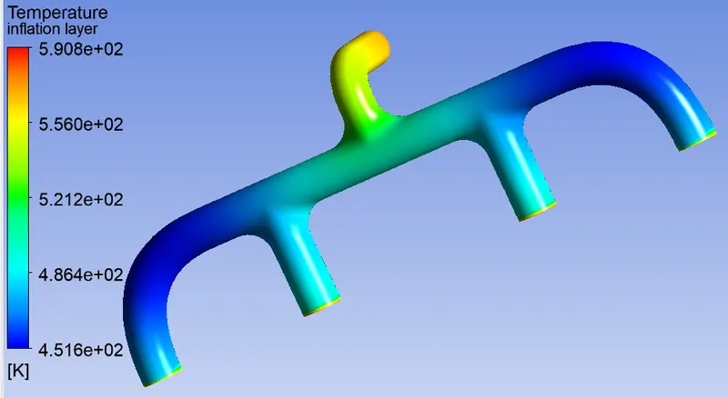
In the above picture, we can see the temperature distribution in the inflation layer. We are getting the maximum temperature at the outlet of the exhaust body. The maximum temperature we got is 590.8 k and the range of the temperature is 451.6 to 590.8 k.

Temperatue at outlet plane

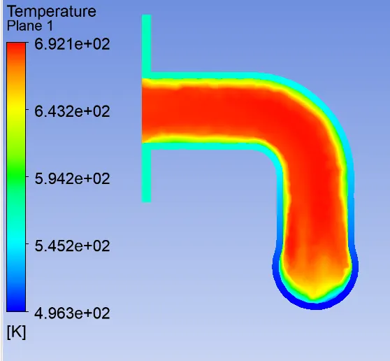
In the above picture, we can see the temperature distribution at the outlet of the exhaust port. The maximum temperature we got is 692.1 k and the range of the temperature is 496.3 to 692.1 k.

Velocity at outlet plane

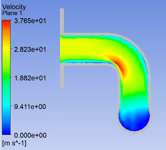
In the above picture, we can see the velocity distribution at the outlet of the exhaust port. The maximum velocity we got is 37.65 m/s and the range of the temperature is 0 to 37.65 m/s.

Temperature at the outer wall

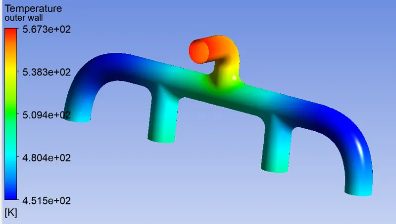
We can see from the above picture that the temperature in the outlet is high on the outer wall.

Case-3

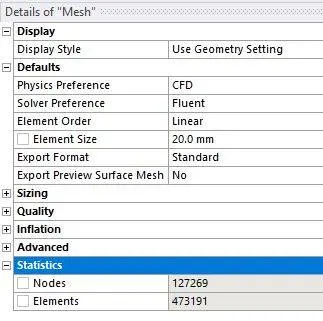
Mesh

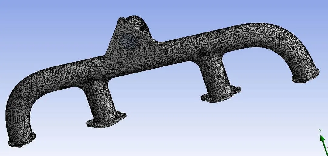
In the finer mesh, I have given the body sizing to the fluid body. I have made it finer so that we can get the HTC value more accurate in the inflation layer.

Heat Transfer Coefficient at the Inflation Layer

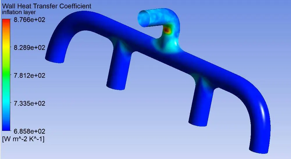
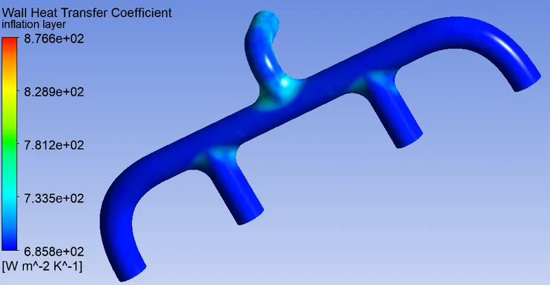
In the above picture we can see the heat transfer coefficient distribution in the inflation layer. The inflation layer is the surface of the internal solid surface in this case which is air. The maximum heat transfer coefficient value we got is 876.6 `Wm^-2K^-1`. The range of the heat transfer coefficient is 685.8 to 876.6 `Wm^-2K^-1`.

We can see from the above plots that at the bend near the outlet, velocity increases because of that there is an increase of the heat transfer coefficient. We got the maximum heat transfer coefficient there.

Temperature at the Inflation Layer

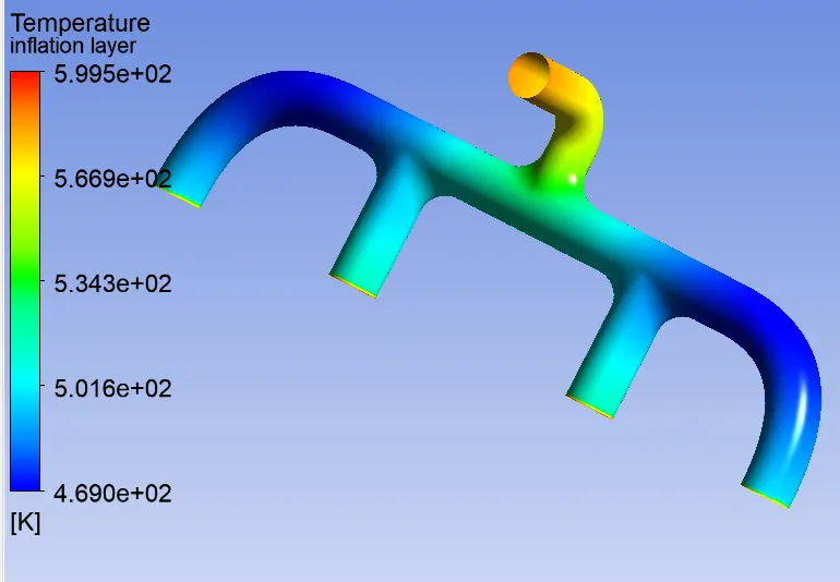
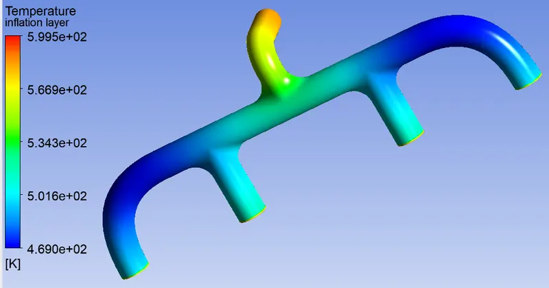
In the above picture, we can see the temperature distribution in the inflation layer. We are getting the maximum temperature at the outlet of the exhaust body. The maximum temperature we got is 599.5 k and the range of the temperature is 451 to 599.5 k.

Temperatue at outlet plane

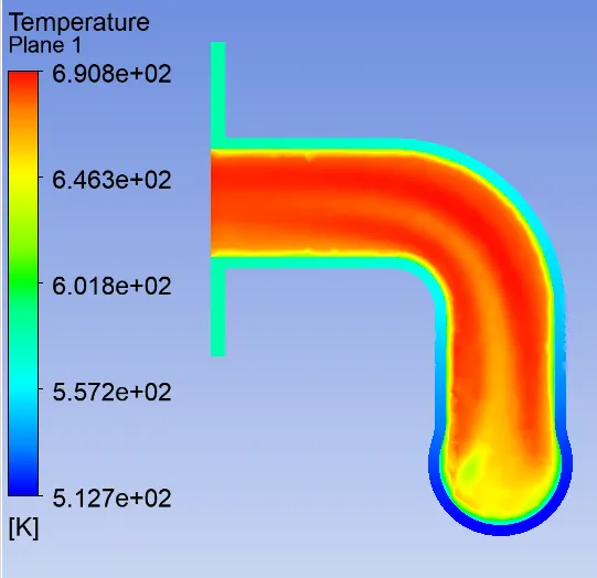
In the above picture, we can see the temperature distribution at the outlet of the exhaust port. The maximum temperature we got is 690.8 k and the range of the temperature is 512.7 to 690.8 k.

Velocity at outlet plane

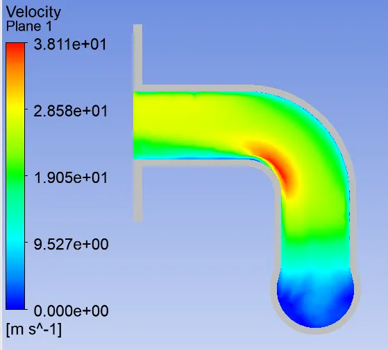
In the above picture, we can see the velocity distribution at the outlet of the exhaust port. The maximum velocity we got is 38.11 m/s and the range of the temperature is 0 to 38.11 m/s.

Temperature at the outer wall

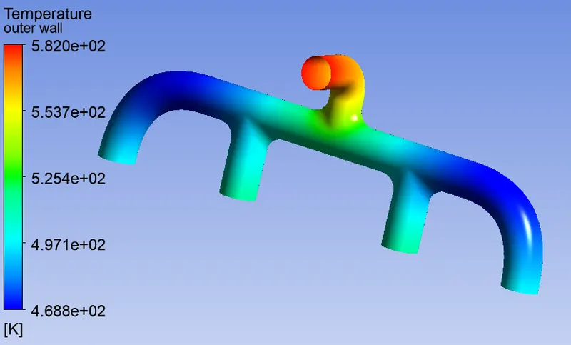
We can see from the above picture that the temperature in the outlet is high on the outer wall.

Grid Independency

For grid independence, we are going to compare the heat transfer coefficient value for different-different mesh sizes.

Case	Mesh Size (mm)	No. of Elements	Maximum Heat Transfer Coefficient in Inflation Layer (`Wm^-2K^-1`)
case-1	Outer Mesh Size = 50 Inner Mesh Size = 50	123395	880.1
case-2	Outer Mesh Size = 30 Inner Mesh Size = 30	130568	869.4
case-3	Outer Mesh Size = 20 Inner Mesh Size = 15	473191	876.6

Conclusion

So From the above table, we can see that the value of heat transfer coefficient for different mesh size they are almost same. There is only small deviation in the values. So we can say that the simulation we have done is right. The grid independence test is a parameter of checking that the simulation we have done is right or wrong. The deviation is very less it is less than 5% so we can say that it passes the grid independence test.

There is no experimental data for this simulation so we can validate by the grid independence test. If it passes the grid independence test then we can say that the result we got is valid or not.

Heat transfer coefficient depends on the area (geometry), temperature, heat transfer rate, the velocity of the fluid and thermal properties of the fluid. So we have to give these values very carefully otherwise we are not going to get the right answer.

We can see from the above plots that at the bend near the outlet, velocity increases because of that there is an increase of the heat transfer coefficient. We got the maximum heat transfer coefficient there.

When air coming from two ways meet, the air velocity increases, and temperature increases in the solid body. Because of that the heat transfer coefficient is also increases in the solid body.