Discretization for range of dx

AIM: Discretization for a range of dx

OBJECTIVE:

In part 1, you had computed the first, second, and fourth-order approximations for a given value of x and dx.

For this program, you need to do the following.

1. For a range of dx, plot the first order, second and fourth-order error.

dx range = [pi/4000,pi/40,20]

Function

`f(x) = (sin(x))/x^3`

first derivative of the function

`f'(x) = (x^3.cos(x)-sin(x).3x^2)/x^6`

`x = pi/3`

dx = linspace(pi/40,pi/4000,20)

CODE:-

clc
clear all
close all

%curve f(x) = sin(x)/x^3;
%Analytical derivative f'(x) = (cos(x)*x^3 - sin(x)*3*x^2)/x^6

x = pi/3;
analytical_derivative = (cos(x)*x^3 - sin(x)*3*x^2)/x^6;

dx = linspace(pi/40,pi/4000,20);

%Numerical derivative
%1st order scheme 
FDS = (sin(x+dx)./(x+dx).^3 - sin(x)/x^3)./dx;

%2n order scheme 
CDS = (sin(x+dx)./(x+dx).^3 - sin(x-dx)./(x-dx).^3)./(2*dx);

%4th order scheme 
FoDS = (sin(x-2*dx)./(x-2*dx).^3 - 8*sin(x-dx)./(x-dx).^3+8*sin(x+dx)./(x+dx).^3-sin(x+2*dx)./(x+2*dx).^3)./(12*dx);

%error calculation
error_FDS = abs(FDS - analytical_derivative);
error_CDS = abs(CDS - analytical_derivative);
error_FoDS = abs(FoDS - analytical_derivative);

%Plotting the results
loglog(dx,error_FDS,'linewidth',3);
hold on
loglog(dx,error_CDS,'linewidth',3);
hold on
loglog(dx,error_FoDS,'linewidth',3);
xlabel('dx')
ylabel('ERROR')
legend('First order','second order','Fourth order')

%Slope claculation 
%calculation the absolute error and dx in term 
first_error_log = log10(FDS);
second_error_log = log10(CDS);
fourth_error_log = log10(FoDS);
dx_log = log10(dx);

% To calculate the slope
slope_1 = diff(first_error_log)./diff(dx_log)
slope_2 = diff(second_error_log)./diff(dx_log)
slope_3 = diff(fourth_error_log)./diff(dx_log)

Code explanation

Here, the given curve function is f(x) = sin(x)/x^3 where the value of x is given as pi/3.

The Analytical derivative of the given function is stated first.

We know that dx's value is being ranged between pi/40 to pi/4000 here.

So we state the range using the linspace command and set the number to values that will be used from the range to 20.

Now, we have to calculate the first-order approximation scheme of the first derivative using the forward differencing method. The value is stored as FDS.

Next, we have to calculate the value of the second-order approximation scheme of the first order using the central differencing method. The value is stored as CDS.

Finally, we have to calculate the value of fourth-order approximation for the first derivative using the central differencing method as well which is stored as FoDS.

Now, we have to calculate the error values for the first, second, and fourth-order approximation by finding out the difference between these values and analytical values.

We are using abs here to find out the absolute value as we know that Y = abs( X ) return the absolute value of each element in array X . If X is complex, abs(X) always returns the complex magnitude.

So, error values for first, second, and fourth-order approximation with the

The next step is to find the slope of the curve, since it is a loglog plot, the absolute error and grid spacing (dx) is converted in terms of log(base10) and storing values to another variable.

Slope between any two point is calculated as, slope = difference in absolute error(in log10)/difference in grid spacing(dx).

OUTPUT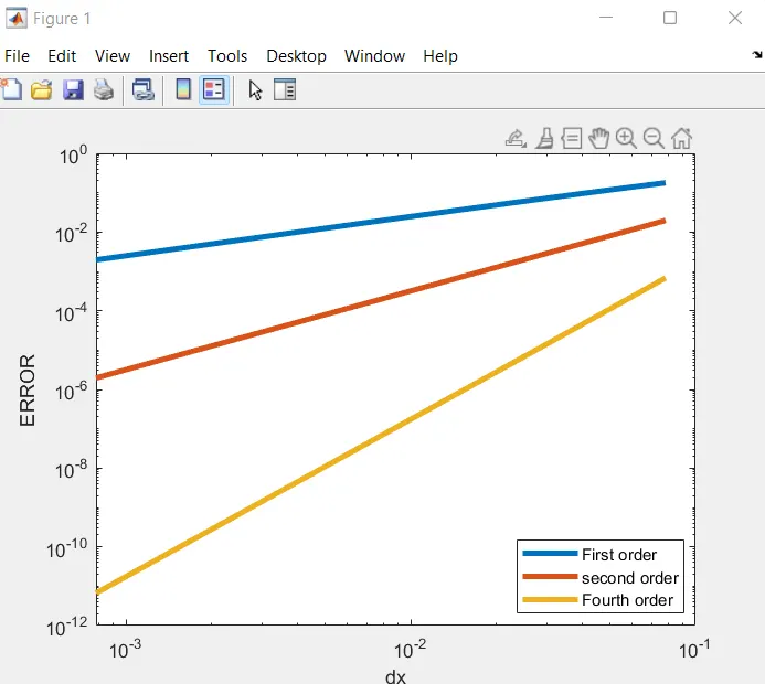

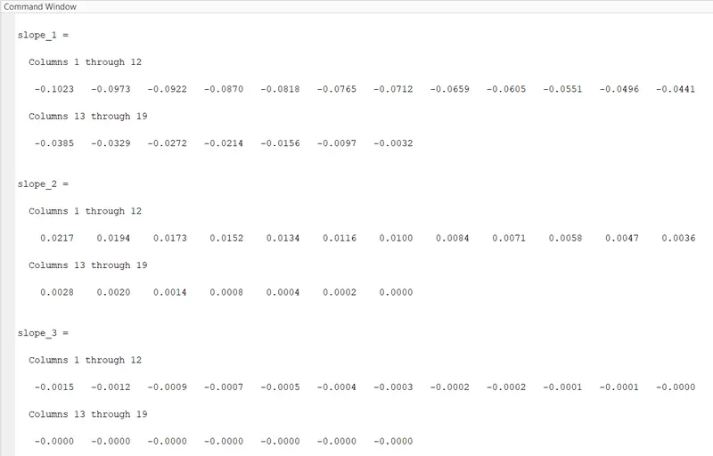
OBSERVATION

By observing the plot we can say that as the value of dx increases the value of absolute error increases exponentially at first as the slope is steeper at first and then it starts to flatten out eventually as the value of dx increases.

The value of error increases gradually in the case of first and second-order approximation but exponentially in the case of fourth-order approximation as the slope of the first-order curve is less steep than the slope of the fourth-order curve which is the steepest.

Here, Higher-order approximations of the function will produce minimal errors and the final value obtained is closer to the analytical value.