Design of Two stage constant ratio reduction power-train

CHAPTER-1 INTRODUCTION:

Scope of the project:

The scope of this project is the Design and Development of a Two Stage Constant Ratio Gearbox to run an All-Terrain Vehicle in SAEINDIA BAJA Endurance.

Figure 1.3 SAEINDIA BAJA Pithampur

SAE BAJA is an ATV Racing Competition, wherein Students from various parts of the country compete each other with their buggies on a rough, rugged, bumpy battlefield with a lot of enthusiasm and passion towards Engineering and Racing.

It is a Platform for Engineering Students to learn and explore the practical aspects and difficulties while building a vehicle and learn good engineering practices that are incorporated by the industries through events like CAE Award, Design Presentation, Cost and Business Pitch event.

With this Context, there are two specific events that influence the design of the powertrain:

1. Sled-Pull: ATV must pull a sled of 2 tons,may be a tractor or a carriage which requires a huge torque.

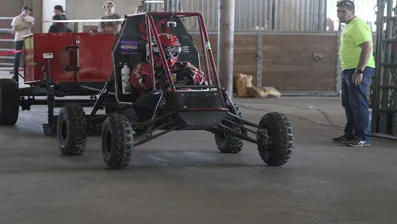
Figure 1.4 Sled Pull

2. Hill-Climb: ATV must negotiate a gradient between 45 to 60 degrees from the ground plane.

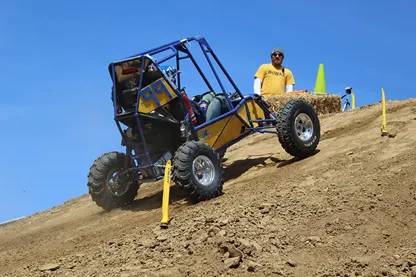
Figure 1.5 Hill Climb

CHAPTER-2 DESIGN CALCULATIONS

2.1 Hill Climb:

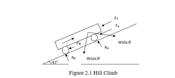
1. Mass of the vehicle (m) = kerb weight + Driver weight

= 175 kg + 60 kg

= 235 kg

2. Earth gravitational pull = 81 n⁄s2
3. Angle of Inclination = 60 degrees
4. Coefficient of rolling resistance (µ) = 0.015
5. Weight distribution (Front : Rear) = 40 : 60
6. Density of air (q) = 1.122 Kg⁄n3
7. Drag Coefficient (c) = 1..08
8. Rear Wheel Radius = 11 inches = 0.2794 m

X Components:

W_v + F_A + F_B + F_d = F

2F_A + W_V + F_d = F equation 1

Y Components:

R_A + R_{B =} W_V

2R_A = W_V

• F_d + W_V+ 2µR_A = F

F_d + W_V + µW_V = F

Ramp angle ( = 60

W_V = 2255.5295 N

C_{d =} 1.08

ρ _air = 1.225 kg/m³

F_{d approx} =

=

= 188.66 m/s²

F_d + W_V + µW_V = F

188.66 + 2255 + 2255 = F

F = 2242.37 N

T = 2242.37 X 0.2794

T = 6206.520 N-m 630 N-m

2403.45 = 152.95

x = 0.085

Hence, the maximum torque required for the propulsion of a 235kg vehicle on a ramp of 60 degrees is 630 N-m.

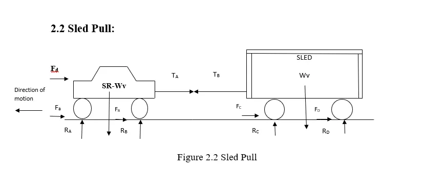
2.2 Sled Pull:

FC = FD

FA = FB

ASSUMPTIONS:

R_A = R_B

R_C = R_D

R_A ≠ R_C

W_L = 2000 kg = 19613.3N

W_v = 230= 2255.5295N

µ = 0.09

X comp:

F_C + F_D - T_B = 0

T_B = 2F_{C Equation} 1

Y comp:

R_C + R_D – W_L = 0

W_L = 2R_{C Equation} 2

Solve equation 1 & 2,

2µR_C – T_B = 0

-2µR_C + µW_L =0

µW_L – T_B = 0

T_B = µW_L

= 0.09 X 19613.3 N

= 1765.197 N

T_B = T_A

Horizontal component – vehicle

F_A + F_B + T_A + F_d = Forward Propulsion

(F_A X 2) + 1765.197 + 188.66 = FP

F_A = µR_A

R_A = =

F_A = 0.09 X 2255.5295

F_A = 202.9976 N

405.99 + 1765.197 + 188.06 = FP

FP = 2359.87447 N

Total forward force needed for thrust against 2 tons

F = 2359.847 N

Torque required T = F x r

= 2359.847 x .2794

= 659.341

660 N-m.

Hence the maximum torque required for the propulsion of the vehicle while pulling a sled of 2tons =660N-m.

2.3 Powertrain Parameters:

Gear tooth and Pitch angle:

Number of Gear pairs=2

Pitch angle of gear = 20 degrees

Total ratio required for propulsion:

Required Torque to be achieved= 660 N-m.

Engine maximum output torque = 19Nm

Ratio required, i = 660/19 =34.73

Ratio of Power Train:

CvTech CVT Maximum ratio = 3.1

j=34.73/3.1=11.20

Splitting j into two parts

Referring standard ratios for spur gears,

j=i1*i2

i1= 3.15

i2= 3.55

Number of teeth of gears in Gear pair 1:

Z1=20

Z2=Z1*i1

Z2=20*3.15 = 63 teeth

Number of teeth of gears in Gear pair 2:

Z3=20

Z4=Z3*i2

Z4=20*3.55 = 71 teeth

Gear Parameters:

Module selected m = 2

Face width= (8-10)*m = 10*m

=10*2= 20mm

Pitch Circle Diameters (PCD):

PCD1=Z1*m

=20*2 = 40mm

PCD2= Z2*m

=63*2= 126mm

PCD3= Z3*m

=20*2= 40mm

PCD4= Z4*m

=71*2= 142mm

Power train Linear Centre to Centre distance (c-c):

c-c=[(PCD1/2) + (PCD2/2) + (PCD3/2) + (PCD4/2)]

= [(40/2) + (126/2) + (40/2) + (142/2)]

= (20+63+20+71)

= 83+91 = 174mm

CHAPTER-3 Modeling and Drafting:

List of components to be designed and assembled:

• 2 Pinions
• 2 Gears
• 3 Shafts
• Power-Train Casing
• Bearings
• Oil Seal
• Snap rings/Circlips
• Engine and Gear Oil

ASSEMBLY:

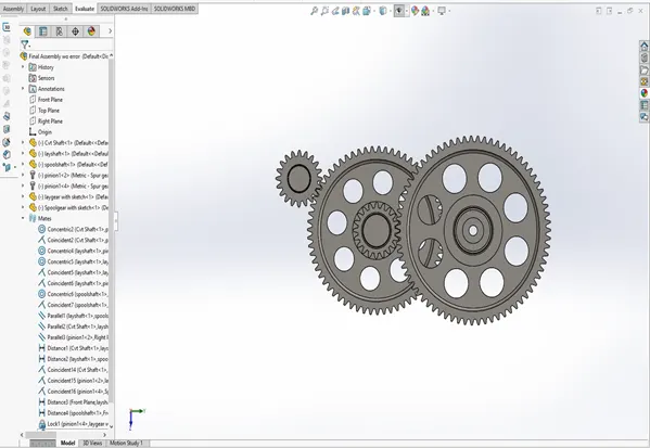
Assembly Front View

Here depicted is the front view of the geartrain, with the following gears & Shafts:

1. Pinion gear connected to the CVT shaft.
2. Lay gear or Intermediate gear connected to Layshaft.
3. Pinion gear on the layshaft to engage the final drive.
4. Spool gear on spool shaft/output shaft.

Power Flow Depiction:

As mentioned above the pairs of gears and shaft engage in a manner as to transfer the output torque from the engine to the wheels.

Let us see how the power flow occurs,

Initially the engine revs up at the starting rpm, meaning idle speed

Then the CVT primary pulley is engaged as the rpm increases, and via the belt drive mechanism, the power is transferred to the secondary pulley, which is connected to the powertrain assembly via input/CVT shaft.

Now, the actual working of gear pairs come into effect, wherein the Pinion transfers torque to Laygear and this in turn makes the second pinion turn the Spool gear to rotate the drive shafts. Then wheels are driven at desired RPM as per torque conversions achieved.

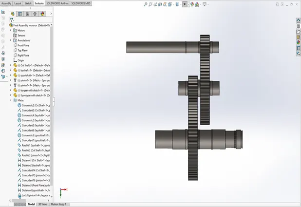
Assembly Power-Flow

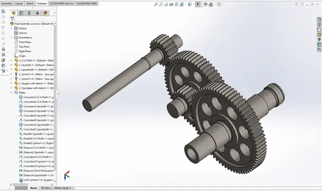
3.6.2 Isometric View of Geartrain assembly:

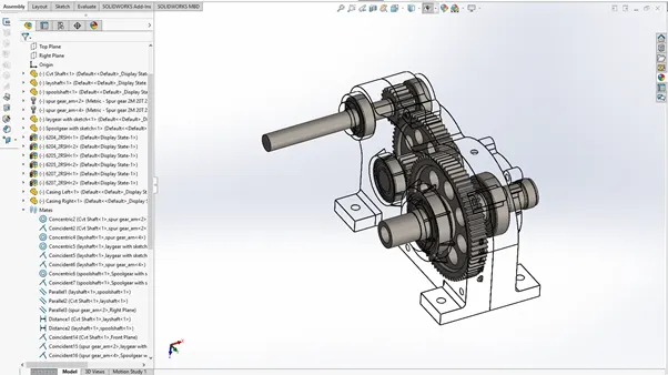
The isometric view is mainly provided here to help visualize how the gears are engaged with each other and also to view how shafts have been designed for retainer rings & bearing mounts.

Assembly Isometric View

Initially after modeling the final Gear train assembly, we move on to the design of casing:

Left and Right sides of the final gearbox is modelled separately and then assembled by means of bolt and nut fasteners.

Outer profile of the casing is drawn based on the alignment of gears on a plane, specifically the vertical plane symmetrical to the vehicle.

Having drawn the outer profile for both the left and right sides, we then move on to give provisions for shafts and bearings.

3.6.3 Assembly of Powertrain and Casing:

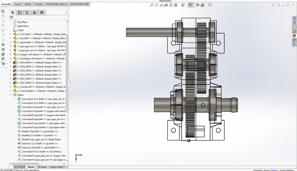
Assembly Top View

Transparent Isometric View

The above two figures depict the assembly of the power-train sub assembly into the casing left and casing right and the seating for bearings and Oil sealants.

3.6.4 Assembly Visualization:

Assembly Visualisation-Isometric View

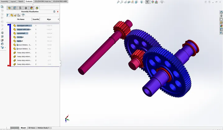
The Assembly Visualization of the powertrain using SOLIDWORKS Analysis shows the weight distribution.

Weight concentration is found to be located at the rear end of the assembly owing to the heavy drive-shaft and spool gear.

Weights of all components of the assembly have been shown in the above figure in decreasing order.

Exploded View of Assembly:

Exploded View-Top

Exploded View-Isometric

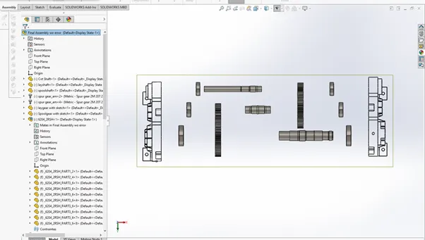
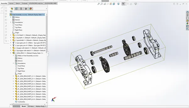
The above two figures show the symmetricity of the assembly and that the shafts are simply supported on either ends via deep groove ball bearings.

CHAPTER 4:DESIGN VALIDATION:

4.1 Analysis of powertrain:

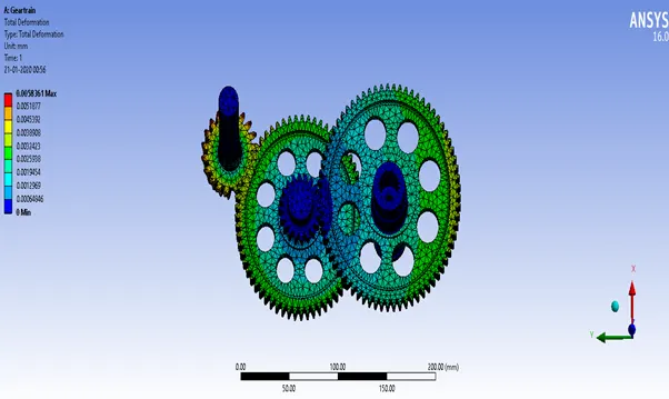
Total Deformation of Powertrain

Structural Analysis was carried out for the powertrain to check the maximum torque it can handle momentarily.

The software used was ANSYS Workbench 16.0.

4.1.1 Boundary Conditions:

No fixtures were determined as all the components were moving in rotary motion.

No-separation type of contact was given between the cylindrical faces of shafts and gears.

4.1.2 Meshing:

All the 6 bodies of the assembly were meshed using tetrahedron mesh elements of size 1mm for maximum accuracy.

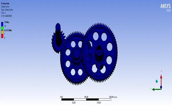
Factor of Safety-Powertrain

4.1.3 Forces:

A moment in the clockwise direction was given to pinion 1 of value 60,000 N-mm, which would be transferred to other gears via pairing and contacts.

4.1.4 Result:

A total deformation of 0.05mm at the tooth region.

A minimum Factor of Safety of 4.57 at the critical region of contact.

4.2 Analysis of Brake Caliper Mount:

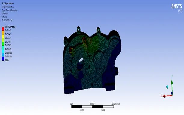
Total Deformation of Mount Tabs

Structural Analysis was carried out for the mount above the bearing of output shaft using ANSYS WORKBENCH 16.0, to test the maximum vertical load and moment the tabs can handle.

Isometric view of the meshed casing is shown above.

4.2.1 Boundary Conditions:

The Gear-Casing Assembly was fixed at its mounting tabs (4 M12 points).

No contact was established as no moving parts are involved.

4.2.2 Meshing:

All the 6 bodies of the assembly were meshed using tetrahedron mesh elements of size 1mm for maximum accuracy.

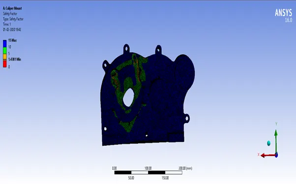
Factor of Safety-Mounting Tabs

4.2.3 Forces:

A moment of 3000 N-mm in the clockwise direction was given to the two tabs and the total deformation was visualized.

4.2.4 Result:

A total deformation of 0.039 mm at the two mounting tabs.

A minimum Factor of Safety of 1.4381 at the critical region of contact.

CHAPTER-5 COMPUTER AIDED MANUFACTURING:

Operation Sequence: -

Setup-1:

Facing

Adaptive Flat end milling

Drilling holes perpendicular to x-plane

Drilling holes perpendicular to y plane

Setup-2:

Facing

2D Adaptive flat end Milling

2D Adaptive boring

Ball end milling for finishing

5.3 CNC Milling:

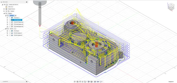
Figure 5.1 CNC Milling Tool Path

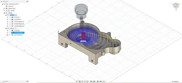
Figure 5.2 2D Adaptive Boring Tool path

Figure 5.1 and 5.2 show the tool path generated for 3D and 2D Adaptive flat end milling using tool 2.

The approximate machining time for this operation is 1hr 29min plus 30min.

This includes multiple rough cuts of each 2mm depth followed by 2 finishing cuts. This operation gives the first outer contour of the part.

5.4 Drilling tool path:

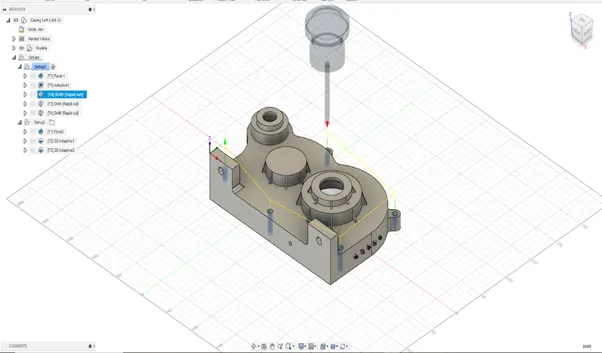
Figure 5.3 Vertical Drilling Tool Path

Figure 5.3 shows the tool path for the 5 mount-tab holes along the x-direction

ACCESSABILITY:

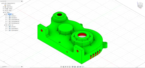
Figure 5.7 Accessibility Analysis Positive z direction

Accessibility analysis was done for both the setups as shown above and below and accessible and non-accessible faces and features were recognized for manufacturability. Plain GREEN shows that all faces required are accessible.

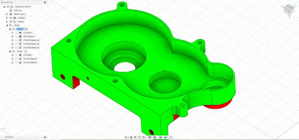
Figure 5.8 Accessibility Analysis Negative z direction

5.7 Minimum and Maximum Radius of Drill tool:

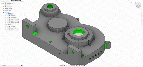
Figure 5.9 Min & Max Radius of Drill Tool, positive z direction

Various holes to be drilled are of varying sizes, Hence the maximum and minimum Radius of the drill size was found

Maximum size-10mm Minimum Size-3mm

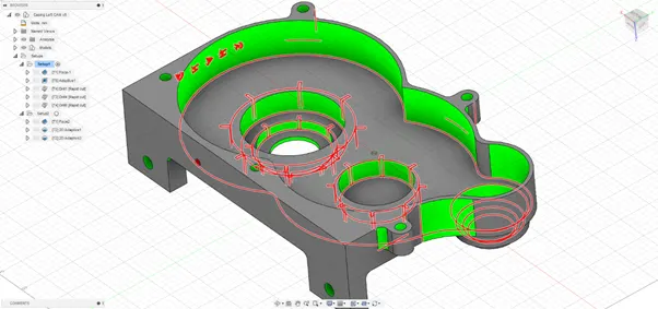
Figure 5.10 Min & Max Radius of Drill Tool, negative z direction

5.8 Sharp Edge Detection:

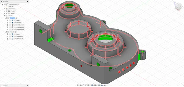
Figure 5.11 Sharp Edge detection

The sharp edges to be resolved and machined are highlighted in red lines in the above figure