Aim:
To write a program to fit a quadratic and cubic polynomial for the Cp data and measure the fitness characteristics for both the curves.
Theory:
What is Curve Fitting?
Curve fitting is the process of constructing a curve, or mathematical functions, which possesses the closest proximity to the real series of data. By curve fitting, we can mathematically construct the functional relationship between the observed dataset and parameter values etc. It is highly effective in the mathematical modelling of some natural processes.
There are 4 parameters that define the goodness of the curve fit. They are:
1. Sum of squares due to errors (SSE)
2. R-Square (R)
3. Adjusted R-Square
4. Root Mean Squared Error (RMSE)
Program Description:
In this program, we are trying to find and plot the graph for finding "specific heat for oxygen as a function of time".
Program 1:
- polyfit - to assign the data into the equation
- polyval - to assign the results obtained from polyval to their corresponding temperature
Program 2:
• A similar program is written to find the best possible curve for the given set of data
• In this program, we have divided it into 8 parts using a "for loop".
Program 1:
%curve fitting by a linear and cubic polynomial for the cp data.
clear all
close all
clc
%load data
cp_data=load('data');
temperature=cp_data(:,1);
cp=cp_data(:,2);
%Curve fit
%cp=a*t^2+b*t+c
figure(1)
coeffs=polyfit(temperature,cp,2);
%polyfit command is to minimalize the difference between the original and predicted data set
predicted_cp=polyval(coeffs,temperature); %predicted data set
%comparing with original dataset
plot(temperature,cp,'linewidth',3); %original dataset
hold on
plot(temperature,predicted_cp,'linewidth',3,'color','r') %predicted dataset
xlabel('Temperature [K]');
ylabel('Specific Heat [KJ/Kmol-K]');
legend('Original dataset','Predicted');
figure(2)
%To plot the graph for 3rd degree equation
coeffs2=polyfit(temperature,cp,3);
predicted_cp2=polyval(coeffs2,temperature);
plot(temperature,cp,'linewidth',3);
hold on
plot(temperature,predicted_cp2,'linewidth',3,'color','g');
xlabel('Temperature [K]');
ylabel('Specific Heat [KJ/Kmol-K]');
legend('Original dataset','Predicted');
Output :
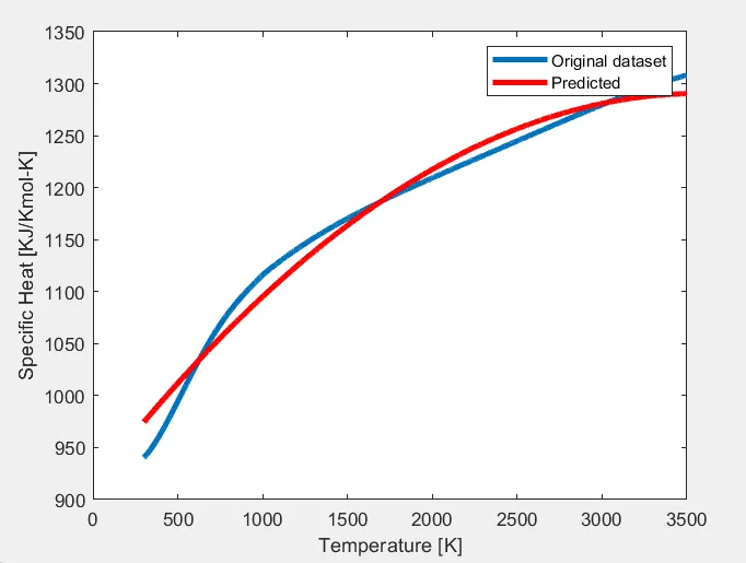
Output graph when degree of polynomial is 2 (the two lines are pretty far)
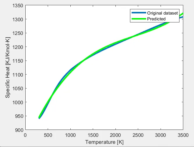
We can make them a bit closer by giving a higher degree.
Output graph when degree of polynomial is 3 (the two lines are almost exact)
But for this program, if we try increasing the degree of polynomial to 3 or more, we get a warning form MATLAB stating that the polynomial is badly conditioned.
Therefore, we have to make changes to the current program in order to not get the warning again.
Program 2:
clear all
close all
clc
cp_data=load('data');
temperature=cp_data(:,1);
cp=cp_data(:,2);
a=1;
b=400;
for i=1:8 % Splitting the graph into 8 parts
coeff=polyfit(temperature(a:b),cp(a:b),3);
predicted_cp(a:b)=polyval(coeff,temperature(a:b));
a=b+1;
b=b+400;
end
plot(temperature, cp, 'color', 'r');
hold on;
plot(temperature, predicted_cp, 'color', 'b');
xlabel('Temperature [K]');
ylabel('Specific Heat [KJ/Kmol-K]');
legend('Actual Cp', 'Curve Fit');
Output :
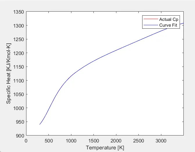
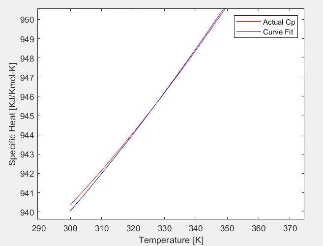
If we zoom in on the graph, it can be seen that two lines blue and red separately.
they look coincidental from far off.
Zoomed figure is shown below :
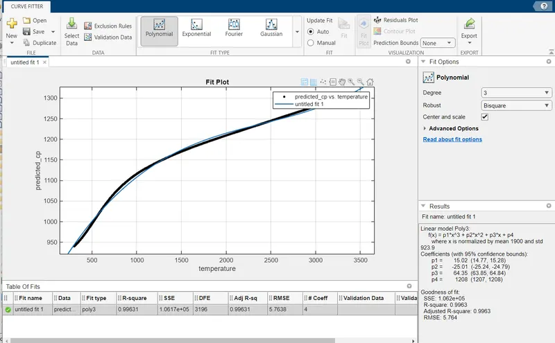
Output from the curve fitting tool :
Here to the bottom left, we can see the four parameters that we had mentioned in the theory section ,
i.e., SSE, R-square, Adjusted R, and RMSE.
Conclusion :
Curve fit was done succesfully for the linear and cubic polynomials.
It was observed that higher the value of polynomial, better the curve fit.