Curve fitting

Aim: - To write a code in MATLAB to fit linear and cubic polynomial for the given specific heat and temperature data.

Objective: - A. To fit the given data into following curves –

1. Linear polynomial
2. Cubic polynomial
3. Fitting different curve in splitwise method
4. To determine the fitness of these curves.

Theory and Equation: -

Curve fitting- It is a process of constructing a curve or a mathematical function to a real series of data with least possible error. it can provide a functional relationship between observed dataset (dependent variable) and parameter values (independent variable).it is highly effective in mathematical modelling of natural process .

Error in curve fitting:- This is the deviation of predicted data to the real data at each individual points.it can be calculated by following formulae

Error= |y(i)−value of f(x) at x(i)|= |y(i)−f(x(i)) |

Parameters used for fitness characterstics of curve: - There are four different way to determine fitness of curve. They are as follow: -

1. The sum of squared error (SSE):- it is the total sum of square of error at each data points.

It is evaluated by following formula: -

SSE(sum of squared errors)= `∑_(i=0)^n( Error (i))^2`

The closer the value to 0 the better fit the curve is.

2.R-square: - the value of R-square can be calculated by: -

`R^2 = (SSR)/(SST)` where SST= SSR+SSE

`SSR= ∑_(i=0)^n((fx(i))-Mean)^2`

The closer its vale to 0 is worst fit and closer to 1 is best fit curve.

3. Adjusted R-square: - It is normalizing the variation in R-square which is due to variation in R-square by an insignificant independent variable. It is calculated by:

`R_adj^2=1-[((1-R^2 )*(n-1))/(n-k-1)]`,

where n is no. of data points and k is no. of independent variable.

4.Root mean squared error(RMSE):- This statistic is also known as the fit standard error and the standard error of the regression. It is an estimate of the standard deviation of the random component in the data, and is defined as,

RMSE=`√((SSE)/n)` , where n is the total number of datapoints available.

The lower the value of RMSE better the fit.

Splitwise method of curve fitting: - it is a method used in higher degree of polynomial of abrupt changes in the data point. In this method the data in divided into smaller sets and each set is fitted individually and then is plotted together, hence increasing the goodness of fit.

To increase the goodness of fit CENTERING AND SCALING is done. In centring we centre the data set around 0 and in scaling, the factor are scaled so as to get better control over change of data with change of parameters.

MATLAB code:-

close all
clear all
clc
%loading data file and assigning each column to respective variable
d= load('data');
temp=d(:,1);
cp=d(:,2);
n=1;
fprintf('the curve fitting of %d degree',n);

subplot(2,1,1)
hold on
%plotting original data
plot(temp,cp,'--','linewidth',3,'color','r');
xlabel('Temperature[K]');
ylabel('Specific heat [KJ/Kmol-k]');

%for linear curve fitting
co_eff=polyfit(temp,cp,n)
p_cp=polyval(co_eff,temp);

%plotting predicted data
plot(temp,p_cp,'linewidth',2,'color','b')
legend("given data","predicted data of 1 degree fit",'location','best')

%calling function to calculate goodness of fit
curve_error(cp,p_cp,n);
%for cubic curve fitting
n=3;
fprintf('\n\nthe curve fitting of %d degree',n);
co_eff3=polyfit(temp,cp,n)
p_cp3=polyval(co_eff3,temp);
subplot(2,1,2)
hold on
%plotting original data
plot(temp,cp,'--','linewidth',3,'color','r');
xlabel('Temperature[K]');
ylabel('Specific heat [KJ/Kmol-k]');
%plotting predicted data
plot(temp,p_cp3,'linewidth',3,'color','g')
legend("given data","predicted data of 3 degree fit",'location','best')
%calling curve error function to determine fitness of curve
curve_error(cp,p_cp3,n)

here the function ployfit is use to calculate the coefficients of the polynomial, which then passed into polyval function with the independent variable to evaluate the dependent variable which in this case is specifi heat.

In the above code a function is called , which is named ‘curve_error’, the body of the function is:-

function [P]= curve_error(cp,p_cp,n)

l=length(cp);

%calculating mean of original data
cp_mean =mean(cp)
%for finding sum of squared error
sse=0;
for i=1:l
    sse=sse+(cp(i)-p_cp(i))^2;
end
fprintf('\nTHE SSE OF %d DEGREE is  %f ', n, sse);

%for finding r_squared value
a=0;
for j=1:l
    a=a+(p_cp(j)- cp_mean)^2;
end
rsqr= a/(a+sse);
fprintf('\nTHE R SQUARE OF %d DEGREE IS %f', n,rsqr);

%for calculating root mean squared error value
rmse=(sse/l)^.5;
fprintf('\nTHE RMSE VALUE OF %d DEGREE IS %f',n,rmse);
end

in this function 3 different criterion is calculated to show the goodness of the fit of the curve so as on can determine the best fit.

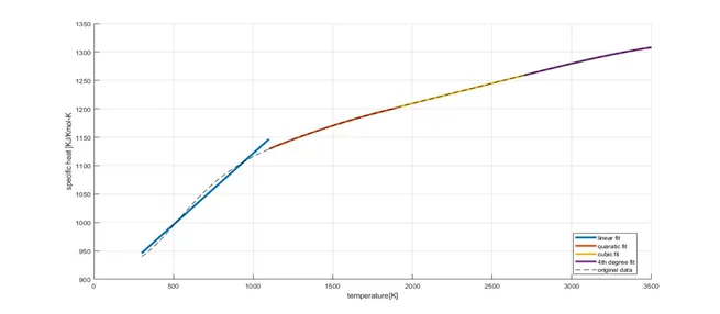
SPLITWISE METHOD FOR CURVE FITTING- the data set is divided into four equal set and each set is treated individualy . the code for this is:-

close all
clear all
clc
%loading original data
d = load('data');
l = length(d);
%dividing the data into four equal parts
temp1=d(1:800,1);
temp2=d(801:1600,1);
temp3=d(1601:2400,1);
temp4=d(2401:3200,1);

cp1=d(1:800,2);
cp2=d(801:1600,2);
cp3=d(1601:2400,2);
cp4=d(2401:3200,2);

%for first data set linear fiting 
coeff1=polyfit(temp1,cp1,1)
p_cp1=polyval(coeff1,temp1);
curve_error(temp1,p_cp1,1)

%FOR 2ND DATA SET QUADRATIC FIT 
coeff2=polyfit(temp2,cp2,2)
p_cp2=polyval(coeff2,temp2);
curve_error(temp2,p_cp2,2)

%for 3rd data set cubic fit with scaling and centring option
[coeff3,S,mu]=polyfit(temp3,cp3,3);
fprintf('\n\ncoeff3 = \n\n%f %f %f %f',coeff3)
%scaling and centring is done
p_cp3=polyval(coeff3,temp3,[],mu);
curve_error(temp3,p_cp3,3)

%for 4th data set curve fitting of 4th degree wit centring and scaling
[coeff4,S,mu]=polyfit(temp4,cp4,4);
fprintf('\n\ncoeff4 = \n\n%f %f %f %f %f',coeff4)
p_cp4=polyval(coeff4,temp4,[],mu);
curve_error(temp4,p_cp4,4)

hold on
plot([temp1,temp2,temp3,temp4],[p_cp1,p_cp2,p_cp3,p_cp4],'linewidth',3)
xlabel('temperature[K]')
ylabel('specific heat [KJ/Kmol-K')
plot([temp1,temp2,temp3,temp4],[cp1,cp2,cp3,cp4],'--','color','k')
legend('linear fit','quaratic fit','cubic fit','4th degree fit','original data','location','best')   
grid on

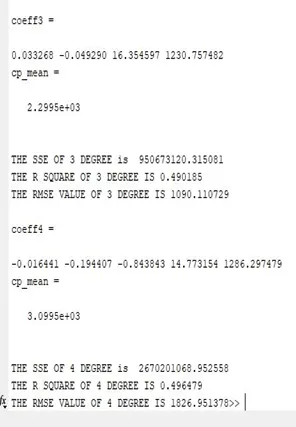
it also uses the same curve_error function to get the goodness of fit.

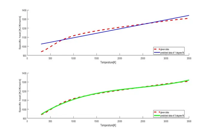
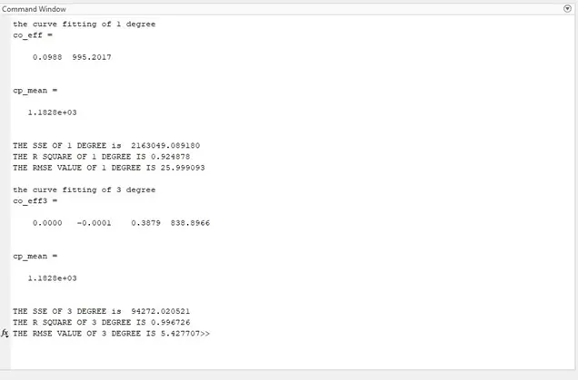
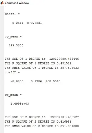
Conclusion: - 1. Between linear fit and cubic fit, the cubic fit is the best fit curve for the cp data. This can be seen the figure as well as in the command window which calculates the different criterion for evaluating the fit.

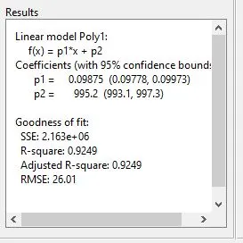
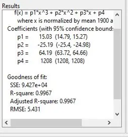
Approximately same values are calculated by MATLAB curve fitting tool for 1^st and 3^rd degree respectively:-

For splitwise method:- The data is divided into four groups hence containing 800 rows each. then each set is treated individually and fitted with linear, quadratic, cubic and 4th degree polynomial respectively.

Inquest: -

Q1. How to make a curve fit perfectly?

Ans: - A curve cold be best fitted by regression techniques with error estimation.

One can zero down errors either by increasing the degree of polynomial or a split wise method could be used i.e. to divided the data into sets and curve fit individually, hence getting a perfectly fit curve for the data.

Q2. How to get the best fit?

Ans: - To get the best fit we can keen on increasing the polynomial degree so as to minise the SSE value of get the R-square value close to 1. We can also divide the data into parts and treat each part individually to get the best fit for them hence reduce errors as a whole.

Q3. What could be done to improve the cubic fit?

Ans: - To improve cubic fit of higher degree fit we can use centering or scaling the data.

In centering the data is centered around o or any other data such as mean and in scaling we multiply the data with a scalor quantity. Splitwise method could also be used.

Refferences:-

1.wikipedia

2.https://projects.skill-lync.com/projects/Curve-Fitting-and-criterion-to-choose-best-fit-41860

3. MATLAB help on polyfit and polyval.