CURVE FIT LINEAR ,CUBIC AND SPLIT-WISE METHOD

AIM :

To write a code to fit a linear and cubic polynomial for the Cp data and plot the linear and cubic fit curves along the raw data points along with titles and lables and to write a code to show splitwise method and to explain the parameters used to measure the fitness characteristic for both the curves.

GOVERNING EQUATION :

Upon finding a curve which satisfies the data points there are 4 quantities which help us measure the goodness of fit criteria or how well the equation is a representing the data points. There are,

• Sum of squares due to error (SSE)
• Sum of squares of the regression (SSR)
• R-square
• Adjusted R-square
• Root mean square error (RSME)

The formula for the respective based on the question :

SSE =`sum` `(`cp - predited_cp`)^2`

SSR = `sum``(`predicted_cp - mean_cp`)^2`

SST = SSE + SSR

R_square = `(SSR)/(SST)`

R_square_adjusted =`1-[((1-R^2)(n-2))/(n-k-1)]`

k = 1(only temperarture is independent variable)

n = lenght of the datapoints (length(cp))

RSME = `sqrt((SSE)/(LENGTH(cp)))`

OBJECTIVE :

1. Write code to fit linear, cubic polynomial and splitwise method for the Cp data.
2. Plot the linear and cubic fit curves along the raw data points along with titles and lables.
3. Explain the parameters used tp measure the fitness characteristics for both the curves.

THEORY :

Curve fitting is the process of constructing a curve, or mathematical function, that has the best fit to a series of data points, possibly subject to constraints. Curve fitting can involve either interpolation, where an exact fit to the data is required, or smoothing, in which a "smooth" function is constructed that approximately fits the data. A related topic is regression analysis, which focuses more on questions of statistical inference such as how much uncertainty is present in a curve that is fit to data observed with random errors. Fitted curves can be used as an aid for data visualization, to infer values of a function where no data are available, and to summarize the relationships among two or more variables. Extrapolation refers to the use of a fitted curve beyond the range of the observed data, and is subject to a degree of uncertaininty since it may reflect the method used to construct the curve as much as it reflects the observed data.

Polynomial curves fitting points generated with a sine function. The black dotted line is the "true" data, the red line is a first degree polynomial, the green line is second degree, the orange line is third degree and the blue line is fourth degree.

PROGRAM :

MATLAB PROGRAM FOR LINEAR FIT CURVE:

clear all
close all
clc

% Preparing the data
cp_data = load('data');
temperature = cp_data(:,1);
cp = cp_data(:,2);


%curvefit 
% cp = a*T + b

co_eff = polyfit(temperature, cp, 1 );
predicted_cp = polyval(co_eff, temperature);

%plotting
plot(temperature,cp,'LineWidth',3)
hold on
plot(temperature, predicted_cp, 'LineWidth',3,'Color','r')
xlabel('temperature [k]')
ylabel('Specific Heat [KJ/Kmol-k]')
legend('original curvefit','predicted linear curvefit','location','northwest')
title('temperature vs specific heat')

%to find [R square] for finding the best fit
%finding mean of cp
total_cp = 0;
for i = 1: length(cp);
    total_cp = total_cp + cp(i)
end

mean_cp = total_cp / 3200;

%to calculate sum of square of the regression(SSR)
SSR = 0;
for j = 1:length(predicted_cp);
    SSR = SSR +(predicted_cp(j)-mean_cp)^2;
end

%to calculate sum of squared errors(SSE)
SSE =0;
for k = 1: length(cp);
    SSE = SSE + (cp(k)- predicted_cp(k))^2;
end

SST = (SSR + SSE) ;

Rsquare_lin = (SSR/SST)
k = 1;
a = (1-Rsquare_lin)*(length(cp)-1);
b = (length(cp)-k-1);
Rsquare_adj_lin = 1 - (a/b) 
RSME = (SSE/(length(cp)))^0.5
if Rsquare_lin >= 0.95
    Result1 = sprintf('Linear Curvefit is Good')
else Result2 = sprintf('Linear Curvefit is Not Good')
end

RESULTS for linear fit curve:

EXPLANATION :

1. Initially the program is started with clear all, close all,clc where it cleares all the previous loaded data and we make sure that the data folder is saved in same folder where the main code of the program is saved.

2. Now we have to bring the data inside the main code so we use 'load()' command and you can see the data loaded in the workspace and assigned to the variable 'cp_data'.

3.Now the data has 2 columns the first column is assigned to 'temperature' and the secomd column is assigned to 'cp'.

4. So for linear polynomial let us take cp=a*t+c is a curve that fits the original data points and have 'cp' and 't' are variables. So to find the exact polynomial we have to find the values of the coefficient of 'a' and constant 'c'.

5. To find value of coefficient we use 'polyfit()'command is used and syntax is

coefficient = polyfit(x,y,n)

In our code, x=temperature, y=cp, n = oder of equation(1)

6.With the coefficient we have found the polynomial and now we evaluate the polynomial with the command 'polyval()' and the syntax is

predicted_values = polyval(coefficient,x)

7. So, since we have used this command we now get predicted values of cp for each value of temperature using this linear polynomial.

8. Now 'plot()' command is used to plot original values of cp to the temperature and plot the predicted values of cp to the temperature and 'hold on' command is used to prevent overwritting of plot command.

9. Now commands like 'xlabel()', 'ylabel()' commands are used to define the x-axis and y-axis and 'title command are used to give title and 'legend()' command are used to differentiate between both the curves.

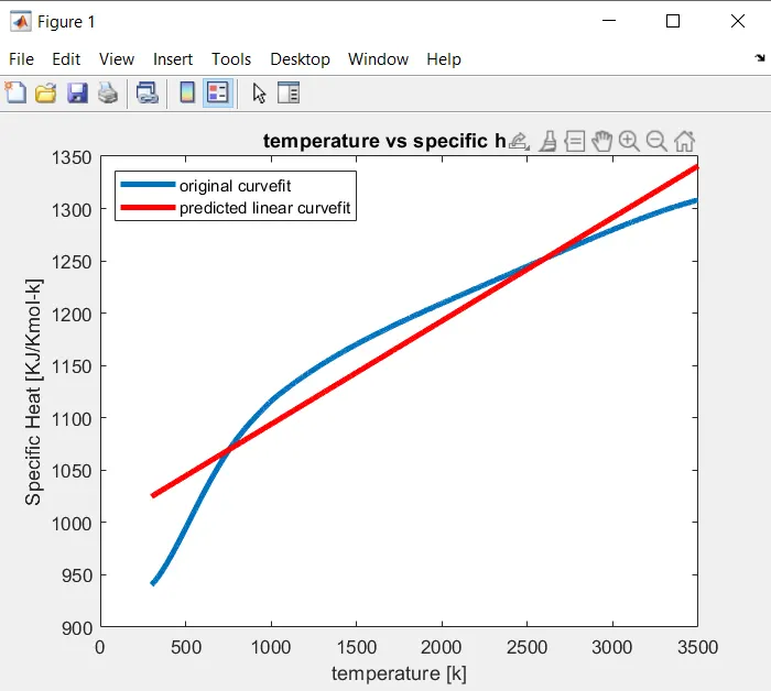
10. We have made a plot that shows the original dataset and curvefit, we can see that the curve fit is not fitting to the original dataset. So to match the bends more correctly we have to increase the order of the curve.

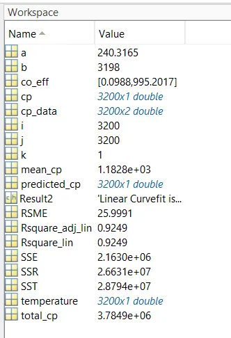
11. To th check the fit of the curvefit we have to find certain values .And these values are calculated with 'for loop' . We have found values of SSE and SSR for each values of cp and also have found valuse of Rsquare, Adjusted Rsquare,RSME also.

12. After doing all the calculation we will get all the values of these terms in the workspace.

13.From the result we got we can say that the value of R_square_lin is 0.9249 which is considered to be not good and the value of RSME is also very high that means the data points are very far away from the curvefit. So by increasing the order of polyomial we can obtain good values of these quantities.

MATLAB PROGRAM FOR CUBIC CURVE FITTING :

clear all
close all
clc

% Preparing the data
cp_data = load('data');
temperature = cp_data(:,1);
cp = cp_data(:,2);


%curvefit 
% cp = a*T^3 + b*T^2+ c*T + d

co_eff = polyfit(temperature, cp, 3 );
predicted_cp = polyval(co_eff, temperature);

%plotting
plot(temperature,cp,'LineWidth',3)
hold on
plot(temperature, predicted_cp, 'LineWidth',3,'Color','r')
xlabel('temperature [k]')
ylabel('Specific Heat [KJ/Kmol-k]')
legend('original curvefit','predicted cubic curvefit','location','northwest')
title('temperature vs specific heat')

%to find [R square] for finding the best fit
%finding mean of cp
total_cp = 0;
for i = 1: length(cp);
    total_cp = total_cp + cp(i)
end

%for i =1:length(cp_data(:,2))
 %   total_cp = total_cp + cp(i)
%end
mean_cp = total_cp / 3200;

%to calculate sum of square of the regression(SSR)
SSR = 0;
for j = 1:length(cp);
    SSR = SSR +(predicted_cp(j)-mean_cp)^2;
end

%to calculate sum of squared errors(SSE)
SSE =0;
for k = 1: length(cp);
    SSE = SSE + (cp(k)- predicted_cp(k))^2;
end

SST = (SSR + SSE) ;

Rsquare_lin = (SSR/SST);
k = 1;
a = (1-Rsquare_lin)*(length(cp)-1);
b = (length(cp)-k-1);
Rsquare_adj_lin = 1 - (a/b) 
RSME = (SSE/(length(cp)))^0.5

if Rsquare_lin >= 0.95
    Result1 = sprintf('Cubic Curvefit is Good')
else Result2 = sprintf('Cubic Curvefit is Not Good')
end

RESULTS for cubic curve fitting :

EXPLANATION :

1. Initially the program is started with clear all, close all,clc where it cleares all the previous loaded data and we make sure that the data folder is saved in same folder where the main code of the program is saved.

2. Now we have to bring the data inside the main code so we use 'load()' command and you can see the data loaded in the workspace and assigned to the variable 'cp_data'.

3.Now the data has 2 columns the first column is assigned to 'temperature' and the secomd column is assigned to 'cp'.

4. So for cubic polynomial let us take cp=a*t^2 + b*t + c is a curve that fits the original data points and have 'cp' and 't' are variables. So to find the exact polynomial we have to find the values of the coefficient of 'a','b' and constant 'c'.

5. To find value of coefficient we use 'polyfit()'command is used and syntax is

coefficient = polyfit(x,y,n)

In our code, x=temperature, y=cp, n = oder of equation(1)

6.With the coefficient we have found the polynomial and now we evaluate the polynomial with the command 'polyval()' and the syntax is

predicted_values = polyval(coefficient,x)

7. So, since we have used this command we now get predicted values of cp for each value of temperature using this cubic polynomial.

8. Now 'plot()' command is used to plot original values of cp to the temperature and plot the predicted values of cp to the temperature and 'hold on' command is used to prevent overwritting of plot command.

9. Now commands like 'xlabel()', 'ylabel()' commands are used to define the x-axis and y-axis and 'title command are used to give title and 'legend()' command are used to differentiate between both the curves.

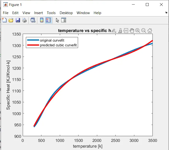
10. We have made a plot that shows the original dataset and curvefit, we can see that the curve fit is fitting ok to the original dataset.

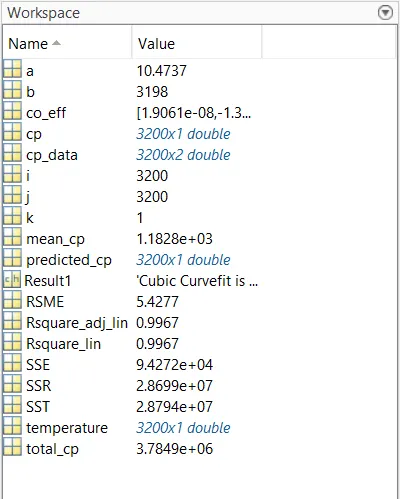
11. To th check the fit of the curvefit we have to find certain values .And these values are calculated with 'for loop' . We have found values of SSE and SSR for each values of cp and also have found valuse of Rsquare, Adjusted Rsquare,RSME also.

12. After doing all the calculation we will get all the values of these terms in the workspace.

13.From the result we got we can say that the value of R_square_lin is 0.9967 which is considered to be good and the value of RSME is also little high that means the data points are very far away from the curvefit. So by increasing the order of polyomial we obtain good values of these quantities.

14. In this using cubic polynomial directly it shows warning symbol due to overfitting of the curve since we have increased the degree of the polynomial so in that case we can use scaling and centering to avoid those warning and produce more accurate results.

15. Using of scaling and centering is not always prefered, instead splitwise method is used tp avoid these warnings. And this method gives more godness of curve for the same polynomial.

PROGRAM FOR SPLIT-WISE METHOD:

clear all
close all
clc

% Preparing the data
cp_data = load('data');
temp = cp_data(:,1);
temp1 = temp(1:800);
temp2 = temp(801:1600);
temp3 = temp(1601:2400);
temp4 = temp(2401:3200);
cp = cp_data(:,2);
cp1 = cp(1:800);
cp2 = cp(801:1600);
cp3 = cp(1601:2400);
cp4 = cp(2401:3200);

%FIRST SET
[co_eff_1,S1,mu1] = polyfit(temp1,cp1,3);
predicted_cp1 = polyval(co_eff_1,temp1,S1,mu1);

for i = 1:length(cp1);
    x1(i) = (cp1(i)-predicted_cp1(i))^2;
    y1(i) = (predicted_cp1(i)-mean(cp1))^2;
end

SSE_1 = sum(x1);
SSR_1 = sum(y1);
R_square_1 = (SSR_1/(SSE_1+SSR_1));
RSME_1 = (SSE_1/length(temp1))^0.5;


%SECOND SET
[co_eff_2,S2,mu2] = polyfit(temp2,cp2,3);
predicted_cp2 = polyval(co_eff_2,temp2,S2,mu2);

for j = 1:length(cp2);
    x2(j) = (cp2(j)-predicted_cp2(j))^2;
    y2(i) = (predicted_cp2(j)-mean(cp2))^2;
end

SSE_2 = sum(x2);
SSR_2 = sum(y2);
R_square_2 = (SSR_2/(SSE_2+SSR_2));
RSME_2 = (SSE_2/length(temp2))^0.5;


%THIRD SET
[co_eff_3,S3,mu3] = polyfit(temp3,cp3,3);
predicted_cp3 = polyval(co_eff_3,temp3,S3,mu3);

for k = 1:length(cp3);
    x3(k) = (cp3(k)-predicted_cp3(k))^2;
    y3(k) = (predicted_cp3(k)-mean(cp3))^2;
end

SSE_3 = sum(x3);
SSR_3 = sum(y3);
R_square_3 = (SSR_3/(SSE_3+SSR_3));
RSME_3 = (SSE_3/length(temp3))^0.5;


%FOURTH SET
[co_eff_4,S4,mu4] = polyfit(temp4,cp4,3);
predicted_cp4 = polyval(co_eff_4,temp4,S4,mu4);

for l = 1:length(cp4);
    x4(l) = (cp4(l)-predicted_cp4(l))^2;
    y4(l) = (predicted_cp4(l)-mean(cp4))^2;
end

SSE_4 = sum(x4);
SSR_4 = sum(y4);
R_square_4 = (SSR_4/(SSE_4+SSR_4));
RSME_4 = (SSE_4/length(temp4))^0.5;

%OVERALL RESULT
R_square_overall = (R_square_1 + R_square_2 + R_square_3 + R_square_4)/4;
RSME_overall = (RSME_1 + RSME_2 + RSME_3 + RSME_4)/4;   


%plotting
plot(temp,cp,'linewidth',7,'color','g')
hold on
plot(temp1,predicted_cp1,'linewidth',3,'color','r')
plot(temp2,predicted_cp2,'linewidth',3,'color','y')
plot(temp3,predicted_cp3,'linewidth',3,'color','b')
plot(temp4,predicted_cp4,'linewidth',3,'color','black')
xlabel('temperature [k]')
ylabel('Specific Heat [KJ/Kmol-k]')
legend('original curvefit','First set','Second set','Third set','Fourth set','location','northwest')
title('SPLIT-WISE METHOD')

RESULT:

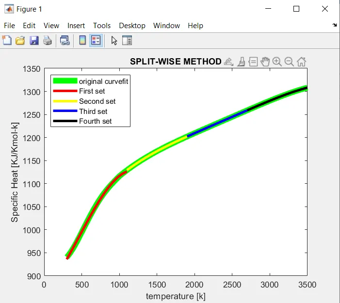
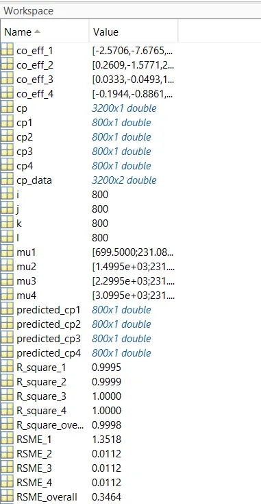
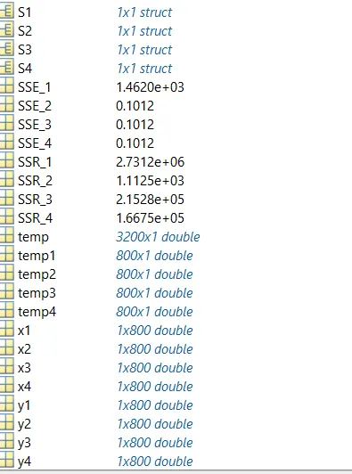
EXPLANATION :

1.In this method we are taking a cubic polynomial let us take cp=a*t^2 + b*t + c is a curve that fits the original data points and have 'cp' and 't' are variables. So to find the exact polynomial we have to find the values of the coefficient of 'a','b' and constant 'c'.

2. The main different is that we are splitting the total data points into four sets of 800 data points and for each part the polynomail coefficient are determined and the polynomail is calculated as it is done foe the previous codes.

3.After doing similar operations as the previous code and when you run the code, the graph obtained will be smoother than the same order polynomail graph that is obtained without splitting the data.

4.Values of R-square, Adjusted R-square, RSME are much better than the previous values obatined without splitting the data.

5. If the data set is further divided into more number of equal sets we will get better values.

1.How to make a curve fit perfectly ?

A perfect fit can always be the best fit but the best bit cannot be a perfect fit always. We can improve perfect fit by minimizing error. In perfect fit, without showing the centering error and scaling error, the curve fit should fit the original curve in that particular order of the polynomial.

2. How to get the best fit ?

The best fit and a perfect fit are two completely phenomena. To get the best fit we can check the parameters for the curve fitting. We can increase the order of the polynomial to get the best fit.

Upon finding a curve which satisfies the data points there are 4 quantities which heph us measure the goodness of fit criteria or how well the equation is a representing the datapoints. They are,

• The sum of squares due to error (SSE)
• R-square
• Adjusted R-square
• Root mean squared error(RSME)

3. What could be done to improve the cubic fit ?

By using the Split-wise method,we can improve the curve fit for the particular order of polynomial. In we are splitting the total data points into equal sets ofdata points and for each part the polynomial coefficient are determined for the curve fit in small ranges. In the last these values are combined to plot over the entire dataset.

Conclusion :

1. In this question, we get three values of R-square for the 3 differfent cases. In the first case, the R-square value for the linear curve fitting is 0.9249 which is less than 0.95, So we conclude that this linear curve fit is not good.

2. So we further increase the order of polynomial to cubic in this the value of R-square for the cubic curve fitting we get 0.9967 which is more than 0.95, so we conclude that this cubic curve fit is good.

3. In the last case we used split-wise method for cubic polynomial, we get R-square value of 0.9998 which is almost equal to 1, So we conclude that this curve is the best fit for the original data set.