Week 4.1 - Genetic Algorithm

• Selection Rules select the individuals, called parents, that contribute to the population at the next generation.

• Crossover Rules combine two parents to form children for the next generation.

• Mutation Rules apply random changes to individual parents to form children.

General concept :

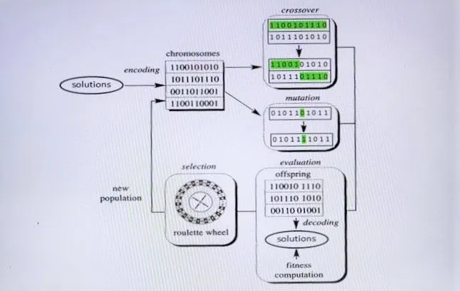
Genetic algorithm starts with an initial set of random solutions called population.

Each individual in the population is called a chromosome representing a solution to the problem at hand.

The chromosomes evolve through successive iterations, called generations.

During each genaration, the chromosomes are evaluated using some measures of fitness.

To crate the next genaration, the new chromosome, called offdprings, are formed by either (a) merging two chromosomes from current generation using crossover operator or (b)modifyinf a chromosome using mutation operator.

A new generation is formed by (a) selecting, according to the sitness values, some pf the parents and offsprings and (b) rejecting others so as to keep the population size constant.

Fitter chromosomes have higher propbabilities of being selected.

After several generations, the algorithms converge to the best chromosome, which hopefully represents the optimum or suboptimum solution to the problem.

Syntax for GA in Matlab :

The format for writing genetic algorithm in MATLAB is as follows:

1. x is the local minima point.
2. fun is the function to be called.(In our case, its the stalagmite function)
3. nvars indicates the no of variables used.
4. A and b are used to indicate any kind inequalities that exist in the function.
5. Aeq and Beq also denotes the inequalities.
6. lb = lower bound.
7. ub = upper bound.
8. nonlcon gives a two vectors representing inequalities and equalities.
9. options is used to perform additional operations like increasing population size. This is done with the help of "optimoptions".

• The satalagmite function is defined separately. This function is later called into the main GA program.
• Now we define the x and y inputs using linspace command.
• Then the input values are transformed into array [xx,yy], so that it can be used to evaluate functions of two variables and plot three-dimensional mesh/surface plots.
• Now the values in the different matrix created can be put as an input into the function that we have created,by calling it. By this we can get the value of the stalagmite function at various values of x and y.
• The total study time is calculated using the 'tic' and 'toc' command at the start and end of the ga for loop respectively.
• Now since we have got the value of the function for various values, Now we need to calculate the maxima value, which can be calculated using the GA command, which is an in-built function in MATLAB.
• Then, the total number of time the GA needs to run is defined using num_cases, and with help of for loop ga is made to run for each iteration and the value is stored in an array.
• GA generally gives the minima value(in built in MATLAB), but we need the maxima hence we can just inverse the stalagmite function by introducing a negative sign.
• The results are then plotted using the surfc command and plot command.
• GA is made to run for 3 iterations, with first iteration having unbounded inputs, second iteration having bounded inputs and third iteration having increasing population size.

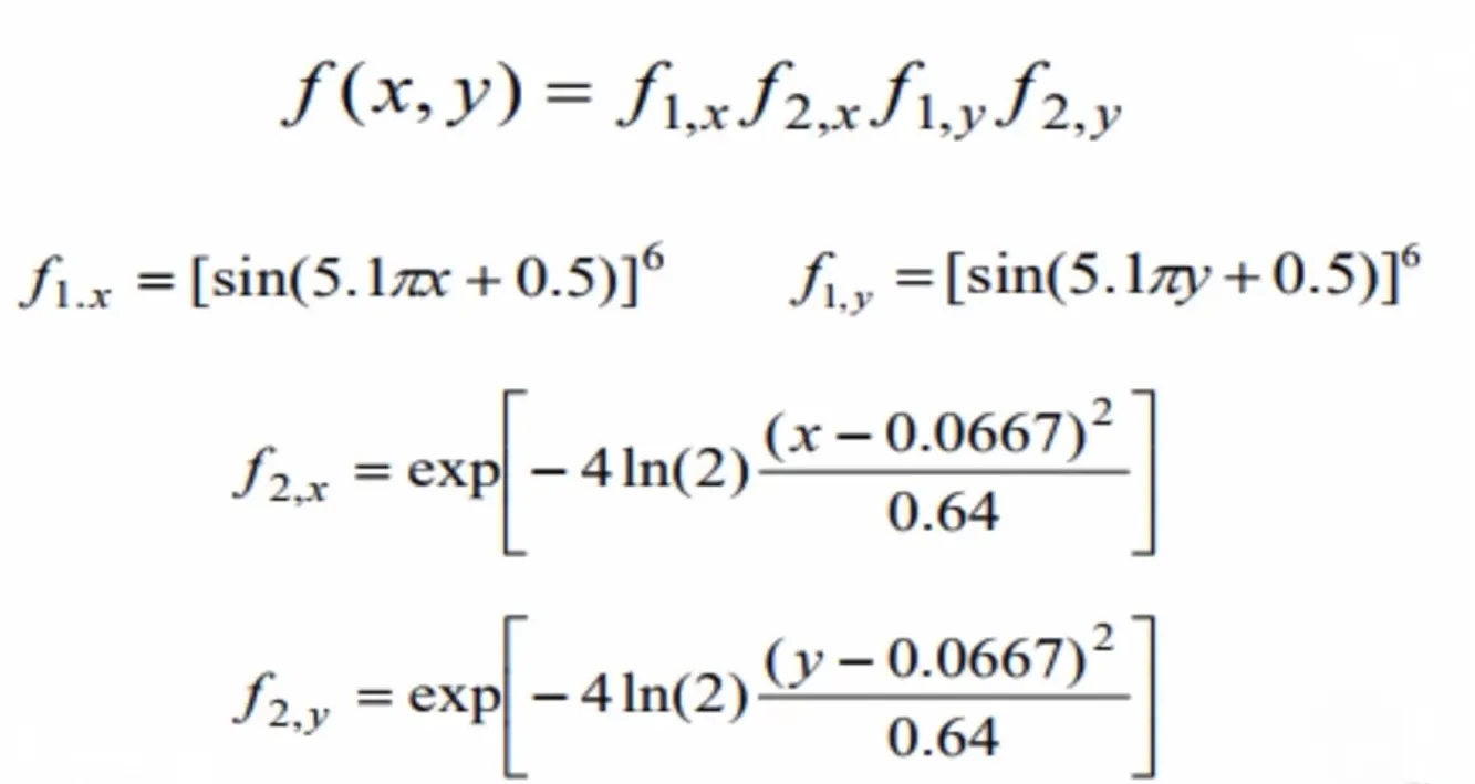
Matlab code for stalamite sunction :

Fitness function :

Matlab code :

function [f] = stalagmite(input_value) 

f_1_x = (sin(5.1*pi*input_value(1) + 0.5))^6;
f_1_y = (sin(5.1*pi*input_value(2) + 0.5))^6;
f_2_x = exp(-4*log(2)*(((input_value(1) - 0.0667)^2)/(0.64)));
f_2_y = exp(-4*log(2)*(((input_value(2) - 0.0667)^2)/(0.64)));

f = -(f_1_x*f_1_y*f_2_x*f_2_y);


end

1. Matlab code for First study (unbounded Inputs) :

STATISTICAL STUDY WITHOUT BOUNDATION

• In this evaluating the optimum value of fitness function at first iteration and calculating it using the geneic algorithm.
• In this code we keep number of iteration as 50.
• Then plotting it into the surf command and also providing the optimum values of the function that how it is varying.
• Also using the tic and tok command to evaluate the time used for optimizing the function.

clear all
close all
clc
% X value inputs
x=linspace(0,0.6,150); 
% Y value inputs
y= linspace(0,0.6,150); 

% No of iteration that GA runs
num_cases=50; 

%Search space is defined but GA Algorithm do not run within the search space
[xx,yy]= meshgrid(x,y);

for i = 1:length(xx);
 for j = 1:length(yy);
 input_value(1)= xx(i,j);
 input_value(2)= yy(i,j);
 f(i,j)= stalagmite(input_value);   
 end
end

% Study Time count start
tic 
for i=1:num_cases;
 % GA syntax is used along with stalagmite function to obtain the optimum
 % values
[inputs,f_opt(i)]= ga(@stalagmite,2);
 x_opt(i)=inputs(1);
 y_opt(i)=inputs(2);
 
end
% Study Time count end
study1_time = toc;
subplot(2,1,1)
hold on
%to create a counter plot(stalagmite 3D cuves) under the surface plot 
surfc(xx,yy,-f) 
xlabel('x-value')
ylabel('y-value')
zlabel('function value')
% To make curve surface without mesh lines 
shading interp  
%plotting the optimum values with a red dot marker along the stalagmite 3D curves
plot3(x_opt,y_opt,-f_opt,'marker','o','markersize',5,'markerfacecolor','r')
title('Unbounded inputs')
subplot(2,1,2)
%plot of f_opt for No.of iteration
%GA gives us Minimum value.So its inverse is taken for Maxima value.
plot(-f_opt) 
xlabel('Number of iterations')
ylabel('Function Maximim')
fprintf ('Study 1 : Unbounded Statistical Behvaiour\n')
fprintf ('The Time taken for the study 1 is : %f\n',study1_time)
fprintf ('The Global Maxima of the Function is : %f\n',-(mean(f_opt)))
sprintf ('optimise value = %f and %f\n',x,y) 

Results :

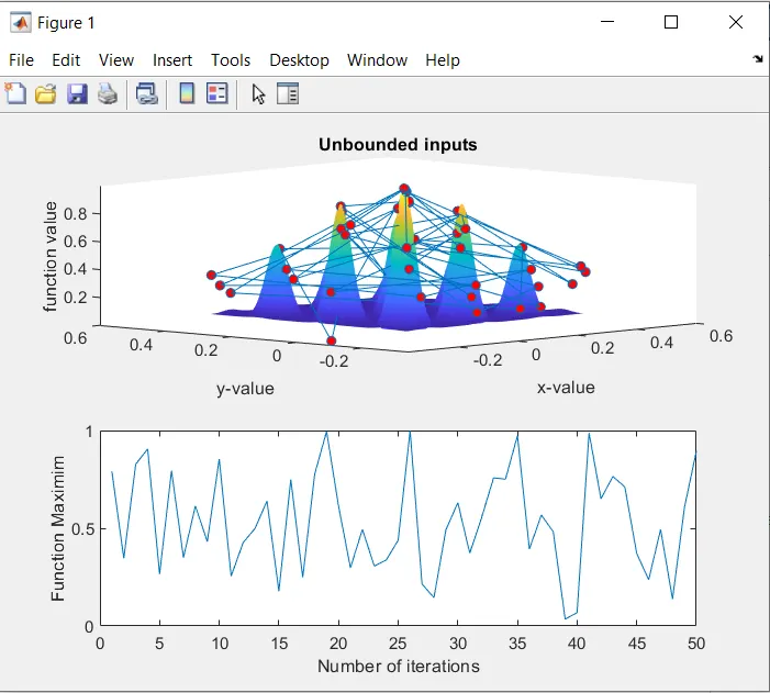
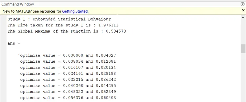
From the figure as shown above it is clear that the results are not that much accurate and giving a lot of variation in optimizing the function.

2. Matlab code for Second study (bounded Inputs) :

STATISTICAL STUDY WITH BOUNDATION

• The difference over here is in providing the upper and the lower limit in the ga so that the search space is reduced with the upper and lower boundary
• In this code we increase the number of iterations to 100.
• And then plotting it as similar to the above study.

clear all
close all
clc

x=linspace(0,0.6,150);  
y= linspace(0,0.6,150);
num_cases=100; % GA runs for 100 iterations
[xx,yy]= meshgrid(x,y);

for i=1:length(xx)
 for j= 1:length(yy)
 input_value(1)= xx(i,j);
 input_value(2)= yy(i,j);
 f(i,j)= stalagmite(input_value); 
 end
end


tic         
for i=1:num_cases;
 % A,B,Aeq and Beq = [],as there is no Linear equalities and inequalities constraints in this function
 % lower boundary of varaibles x and y in ga alogorithmn is set as [0,0]
 % upper boundary of varaibles x and y in ga alogorithmn is set as [0.3,0.3]
 [inputs,f_opt(i)]= ga(@stalagmite,2,[],[],[],[],[0,0],[0.3,0.3]);
 x_opt(i)=inputs(1);
 y_opt(i)=inputs(2);
 
end
study2_time = toc  
subplot(2,1,1)
hold on
surfc(xx,yy,-f)
xlabel('x-value')
ylabel('y-value')
zlabel('function value')
shading interp 
plot3(x_opt,y_opt,-f_opt,'marker','o','markersize',5,'markerfacecolor','r')
title(' With Bounded inputs')
subplot(2,1,2)
plot(-f_opt) 
xlabel('Number of iterations')
ylabel('Function Maximum')
fprintf ('Study 2 : Unbounded Statistical Behvaiour\n')
fprintf ('The Time taken for the study 2 is : %f\n',study2_time)
fprintf ('The Global Maxima of the Function is : %f\n',-(mean(f_opt)))
sprintf ('optimise value = %f and %f\n',x,y) 

Results :

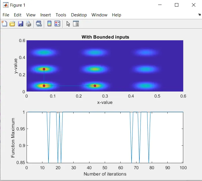
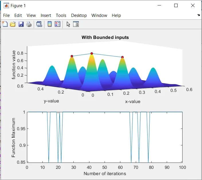
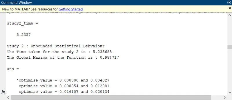
• It is clearly seen from the above that after providing the boundary limits the variation in the optimum value of the function has reduced.

3. Matlab code for Third study (bounded Inputs with increase in population size) :

• In this study using the ‘optimoptions’ command to increase the size of population.
• In this study we further increase the number of iterations to 150.
• The benefit of that will be it will be working on the large set of numbers and which will be led to increase the possibilities of finding the better fitness of the function.
• The drawback is that the time for evaluation will increase.

clear all
close all
clc

x=linspace(0,0.6,150);
y= linspace(0,0.6,150);
num_cases=150; % GA runs for 150 iterations
[xx,yy]= meshgrid(x,y);

for i=1:length(xx)
 for j= 1:length(yy)
 input_value(1)= xx(i,j);
 input_value(2)= yy(i,j);
 f(i,j)= stalagmite(input_value);
 end
end



options= optimoptions('ga');
options= optimoptions(options,'PopulationSize',500);
tic  % Study Time start
for i=1:num_cases
 % Objective function is stalagmite and the number of varaibles is 2
 % A,B,Aeq and Beq = [],as there is no Linear equalities and inequalities constraints in this function
 % lower boundary of varaibles x and y in ga alogorithmn is set as [0,0]
 % upper boundary of varaibles x and y in ga alogorithmn is set as [0.3,0.3]
 % population size is defined by using options in the algorithmn
 [inputs,f_opt(i)]= ga(@stalagmite,2,[],[],[],[],[0,0],[0.3,0.3],[],options);
 x_opt(i)=inputs(1);
 y_opt(i)=inputs(2);
 
end

Study3_time = toc   
subplot(2,1,1)
hold on
surfc(xx,yy,-f)
xlabel('x-value')
ylabel('y-value')
zlabel('function value')
shading interp 
plot3(x_opt,y_opt,-f_opt,'marker','o','markersize',5,'markerfacecolor','r')
title('Bounded inputs with increased population size')
subplot(2,1,2)
plot(-f_opt) 
xlabel('Number of iterations')
ylabel('Function Maximum')
fprintf ('Study 3 : Unbounded Statistical Behvaiour\n')
fprintf ('The Time taken for the study 3 is : %f\n',Study3_time)
fprintf ('The Global Maxima of the Function is : %f\n',-(mean(f_opt)))
sprintf ('optimise value = %f and %f\n',x,y) 

Results :

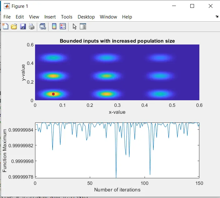
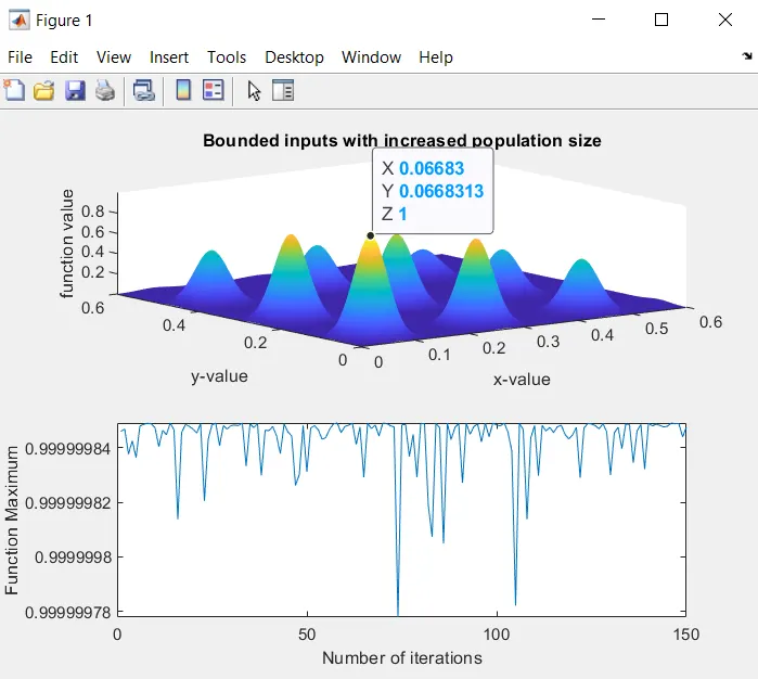
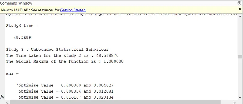
In this case we are getting the optimised value of global maxima with accurate range, since we increased the number of iterations and population size.

Conclusions :

Study 1 :

It can be seen that since the inputs are boundless GA algorithm has mapped local maxima points outside our stalagmite function. Also we cannot get a particular value of global maxima from the graph, and it is hence pointless.

The study time is very less as the GA algorithm is made only to run for 50 iterations.

Study 2 :

The graph is more clear and optimised compared to the 1st iteration since here the bounds were defined and we could get only the values within our range. We are now more clear on the range within which our maxima lies.

Study 3 :

In this case we are getting the optimised value of global maxima with accurate range, since we increased the number of iterations and population size.

Since the number of iterations and population size is increased the study time is so high compared to the previous two iterations.

Thus it can be concluded that GA gives more accurate results in case of bounded inputs and by increasing the number of iterations and population size.

We can conclude that even if we define a particular search space for GA, the GA doesn't run inside the search space. Only in cases of bounded inputs we can get useful results.