Second Order ODE for Simple Pendulum Using MATLAB

Aim :

• To simulate the transient behaviour of a simple pendulum using second order ODE's
• To create an animation of it's motion using MATLAB software.

Governing Equation :

• In mathematics, an ordinary differential equation is a differential equation containing one or more functions of one independent variable and the derivatives of those functions.
• In Engineering, ODE is used to describe the transient behaviour of a simple pendulum.
• The way the pendulum moves depends on the Newtons second law. When this law is written down, we get a second order Ordinary Differential Equation that describes the position of the "ball" w.r.t time.

The second-order ode for simple pendulum is represented as,

`(d^2θ)/dt^2+b/m.dθ/dt+g/lsinθ=0`

where; b = damping coefficient 0.05,

m = mass of ball 1 kg,

g = acceleration due to gravity 9.81 m/s^2,

l = length of the string 1 metre.

Objective :

• To solve ODE which represents equation motion of simple pendulum with damping with help of MATLAB code.
• Plotting the graph of variation of angular displacements vs time , variation of angular velocity vs time.
• Creating the animation plot of for motion of pendulum between motion between 0-20 sec, for angular displacement=0,angular velocity=3 rad/sec at time t=0.

Theory :

Simple Pendulum:

A pendulum is a weight suspended from a pivot so that it can swing freely.When a pendulum is displaced sideways from its resting, equilibrium position, it is subject to a restoring force due to gravity that will accelerate it back toward the equilibrium position. When released, the restoring force acting on the pendulum's mass causes it to oscillate about the equilibrium position, swinging back and forth. The time for one complete cycle, a left swing and a right swing, is called the period. The period depends on the length of the pendulum and also to a slight degree on the amplitude, the width of the pendulum's swing.

Matlab code for simple pendulum :

clear all 
close all
clc

b = 0.05;
g = 9.81;
l = 1;
m = 1;

%initial conditon
theta_0 = [0,3];

%time points
t_span = linspace(0,20,500);

%solve ode
[t, result] = ode45(@(t, theta)ode_func(t, theta, b,g,l,m),t_span, theta_0);

plot(t, result(:,1))
hold on
plot(t, result(:,2))
ylabel('plot')
xlabel('time')

angular_displacement = result(:,1);
ct = 1;
for i = 1:length(angular_displacement);
    angle = angular_displacement(i);
    figure(2)
    title('simple pendulum')
    x0 = 0;
    y0 = 0;

    x1 = l*sin(angle);
    y1 = -l*cos(angle);

    plot([-1.1 1.1],[0 0],'linewidth',2);
    hold on
    plot([x0 x1],[y0 y1],'linewidth',3,'Color','r');
    plot(x1,y1,'o','Markersize',25,'Markerfacecolor','black');
    grid on
    hold off
    axis([-2 2 -2 2])
   % pause(0.001)

    M(ct) = getframe(gcf);
    ct = ct + 1;
end

movie(M);
Videofile = VideoWriter('simple_pendulum.avi');
open(Videofile);
writeVideo(Videofile,M);
close(Videofile);

Matlab code for ODE function :

function [dtheta_dt] = ode_func(t, theta, b,g,l,m)

theta1 = theta(1)
theta2 = theta(2)
dtheta1_dt = theta2
dtheta2_dt = -(b/m)*theta2 - (g/l)*sin(theta1);
dtheta_dt = [ dtheta1_dt ; dtheta2_dt]
end

Explanation of the Matlab code :

• In the main program, initially the inputs such as mass of the bob, length of the string, acceleration due to gravity and damping coefficient are declared.
• Then initial conditions of angular displacement and angular velocity are also given.
• Time period is declared using the 'linspace' function to get multiple time points.
• The ode_pendulum function is then called using ode45 a matlab solver for ode functions
• Now under the for loop we define the coordinates (x0, y0) and (x1, y1)using the equations.
• Both for loops are then ended and the syntax for movie is written.
• The plot command is used to plot the links on the graph. And to animate the plot, getframe command is used. The frame is a snap of the current axes or figure and the counter variable is incremented.

RESULTS :

The graph shows Time Vs displacement (blue) and time Vs Angular velocity(red) as shown in graph,

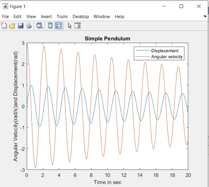
From above graph it can be observed that oscillation of pendulum are gradually damped as we can observe that angulalar displacement and angular velocity was gradually decreasing with time.

ANIMATION FOR SIMPLE PENDULUM :

A youtube link is provided for the animation of simple pendulum using matlab

https://youtu.be/aQTqOprCK94

Due to damping, the pendulum's angular amplitude decreases over time due to the total energy of the pendulum is being transferred to the surrounding environment.

Conclusion :

• We have understood how to solve a second ODEs using MATLAB
• Motion of simple pendulum has been animated sucessfully.