COMBINED SLIP BRUSH TIRE MODEL USING MATLAB

This project aims at modelling the combined slip brush tire models for variable and constant slip angles. The relationship between the lateral force and longitudinal force is projected to the slip angles. We will even see the variation of effective cornering stiffness to the variable slip ratios.

A tire model is a mathematical or an empirical representation of the mechanism through which the tire generates forces and moments in response to inputs such as slip angle and camber angle.

Combined Slip Condition:

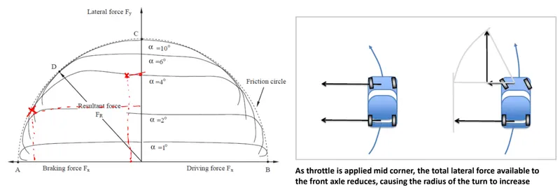
A typical braking-cornering scenario:

Unlike the independent brush tire model scenario, in reality, both braking and cornering forces occur simultaneously during vehicle manoeuvres like a brake in turn and trailing throttle cornering. Therefore a tire model must be able to deal with combined tractive and cornering forces, a situation known as comprehensive slip.

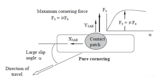
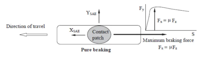
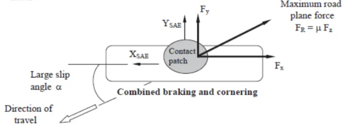
The peak value of the resultant cornering and tractive forces is governed by a curve of radius μFz. This curve is known as the friction circle or the friction ellipse as some tires have more capability in traction or cornering.

The combined brush tire model is conceptualized in the following three regions:

1. Adhesion region:

Longitudinal force: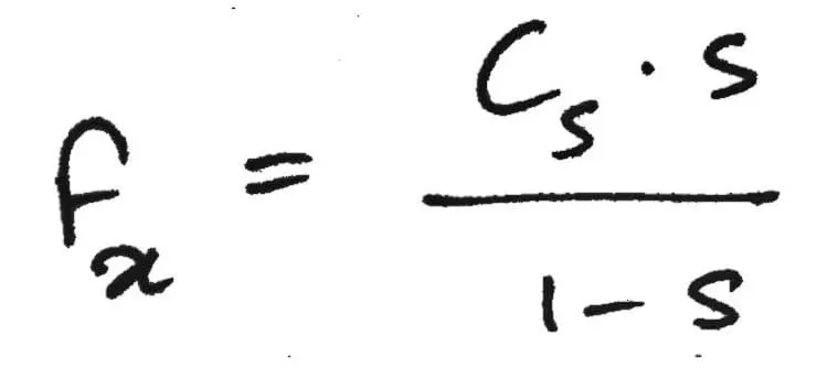

Lateral force: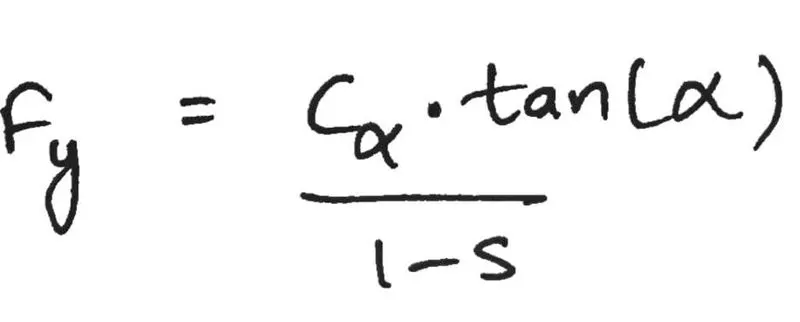

where,

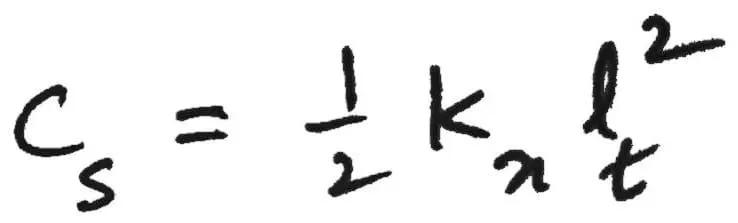, Longitudinal stiffness in N.m^2

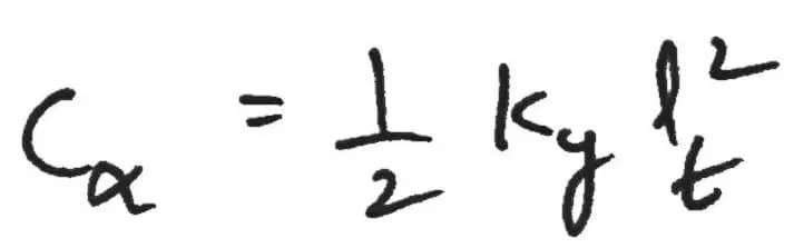, Cornering stiffness in N.m^2

`l_t`: Length of contact patch in m

s: Slip ratio

2. Critical point:

Critical length: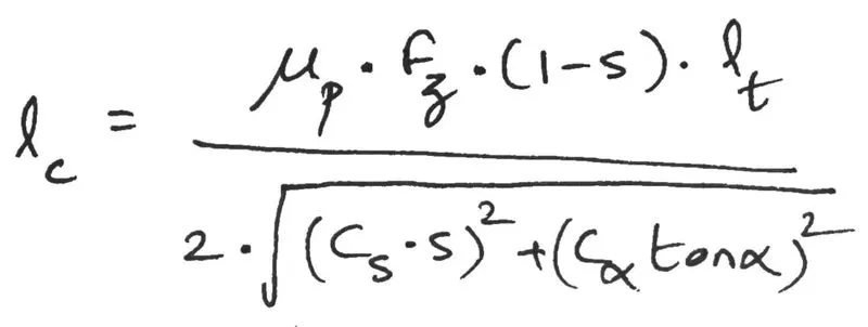

where,

`mu_p`: Peak road-tire friction coefficient

`F_z`: Normal load in N

3. Sliding region:

Longitudinal force: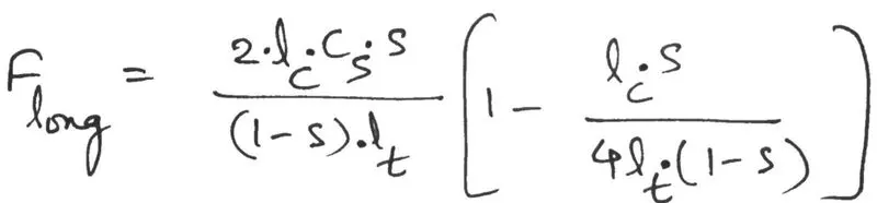

Lateral force: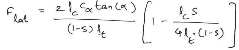

COMBINED SLIP:

Aim:

To plot to show the effect of different slip angles on Lateral force 'Fx' vs Longitudinal force 'Fy'.

Input data:

Slip range = 0 to 1 (or 0 to 100%)

Slip angle = 2, 4, 6, 8, 10 degrees

MATLAB Code:

clear all
close all
clc

Fz = 4000; % Normal load 'N'
u = 0.85; % Coefficient of friction
lt = 0.2; % Length of contact patch in 'm'
kx = 3.5e6; % Tire tangential stiffness per unit length 'N/m^2'
ky = 2.5e6; % Tire lateral stiffness per unit length 'N/m^2'

cs = 0.5*kx*lt^2; % Longitudinal stiffness
ca = 0.5*ky*lt^2; % Cornering stiffness

sr = zeros(); Fx = zeros(); Fy = zeros(); term = zeros(); lc = zeros();
for i = 2:2:10
    sa = deg2rad(i); % Slip angle in radians
    for j = 1:101
        sr(i) = (j-1)*0.01; % Slip ratio
        s = sr(i); 
        term(j) = ((cs*s)^2+(ca*tan(sa))^2)^0.5; % Temporary term
        lc(j) = (u*Fz*(1-s)*lt)/(2*term(j)); % Critical length
        
        if lt <= lc(j) % Adhession region
            Fx(i) = cs*s/(1-s); % Longitudinal force
            Fy(j) = ca*tan(sa)/(1-s); % Lateral force
        else % Slip region
            Fx(j) = (u*Fz*cs*s/term(j))*((1-u*Fz*(1-s)/(4*term(j))));
            Fy(j) = (u*Fz*ca*tan(sa)/term(j))*((1-u*Fz*(1-s)/(4*term(j))));
        end
    end
    
    figure(1)
    plot(Fx,Fy,'Linewidth',1.5)
    hold on
end
    grid on
    xlabel('Longitudinal Force Fx in N')
    ylabel('Lateral Force Fy in N')
    title('Fx VS Fy for different slip angles')
    legend('2 deg','4 deg','6 deg','8 deg','10 deg')

Plots:

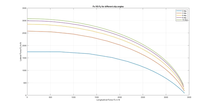
Inference from the plot:

1. The Longitudinal force increases with a decrease in the lateral force for any slip angle.
2. With an increase in the slip angle values, the later force increases. But, the range of longitudinal force remains the same.
3. With an increase in the slip angle, the difference between consecutive lateral forces decrease. This is because the tires start to saturate at higher slip angles.

COMBINED SLIP (ABS AND SIDE FORCE):

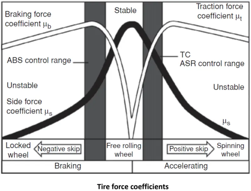
Anti-lock brake systems and traction control systems aim not only to avoid wheel lockup or spin but also to maintain wheel slip near an optimal
value, which achieves maximum possible tire longitudinal forces and in the meantime, avoids a significant reduction in lateral forces.

Aim:

To calculate the effective cornering stiffness and plot to show the effect of different slip angles on Lateral force 'Fx' vs Longitudinal force 'Fy' under different slip ratios and fixed slip angles.

Input data:

Slip ratios = 0, 0.15, 1

MATLAB Code:

clear all
close all
clc

format short
Fz = 3000; % Normal load 'N'
u = 0.8; % Coefficient of friction
lt = 0.2; % Length of contact patch in 'm'
kx = 4e6; % Tire tangential stiffness per unit length 'N/m^2'
ky = 2.275e6; % Tire lateral stiffness per unit length 'N/m^2'
sa = 3;

cs = 0.5*kx*lt^2; % Longitudinal stiffness
ca = 0.5*ky*lt^2; % Cornering stiffness

sr = zeros(); Fx = zeros(); Fy = zeros(); term = zeros(); lc = zeros(); C_eff = zeros();

for j = 1:101
    sr(j) = (j-1)/100; % Slip ratio
    s = sr(j); 
    term(j) = ((cs*s)^2+(ca*tan(sa))^2)^0.5; % Temporary term
    lc(j) = (u*Fz*(1-s)*lt)/(2*term(j)); % Critical length

    if lt <= lc(j) % Adhession region
        Fx(j) = cs*s/(1-s); % Longitudinal force
        Fy(j) = ca*tan(sa)/(1-s); % Lateral force
        C_eff(j) = Fy(j)/sa;
        if s == 0.00 || s == 0.15 || s == 1.00
            fprintf('Effective cornering stiffness = %0.2f N/rad at a Slip ratio of %0.2fn',C_eff(j),s);
        end
    else % Slip region
        Fx(j) = (u*Fz*cs*s/term(j))*((1-u*Fz*(1-s)/(4*term(j))));
        Fy(j) = (u*Fz*ca*tan(sa)/term(j))*((1-u*Fz*(1-s)/(4*term(j))));
        C_eff(j) = Fy(j)/sa;
        if s == 0.00 || s == 0.15 || s == 1.00
            fprintf('Effective cornering stiffness = %0.2f N/rad at a Slip ratio of %0.2fn',C_eff(j),s);
        end
    end
end

    figure()
    subplot(1,2,1)
    plot(Fx,Fy,'Linewidth',1.5)
    grid on
    xlabel('Longitudinal Force Fx in N')
    ylabel('Lateral Force Fy in N')
    title('Fx VS Fy for different slip ratios')
    subplot(1,2,2)
    plot(sr,C_eff,'Linewidth',1.5)
    grid on
    xlabel('Slip ratio')
    ylabel('Effective cornering stiffness C_eff in N/rad')
    title('Slip ratio VS Effective cornering stiffness for different slip ratios')

Effective cornering stiffness values:

Plots:

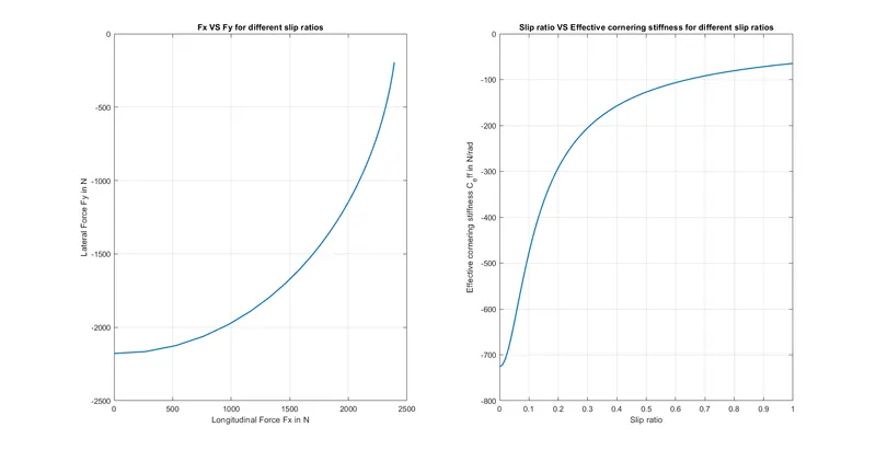
Inference from the plots:

Plot 1:

• The longitudinal force exponentially increases while the lateral force decreases.
• As the slip ratio reaches 1, the longitudinal force saturates. Any change in lateral force won't change it.

Plot 2:

• The effective cornering stiffness drastically increases to a slip ratio of 0.3. Post which, it starts to even out. This is because the tires start to saturate at higher slip angles.