Calculating drag force against a cyclist using MATLAB

AIM : To calculate drag force against a cyclist using MATLAB.

THEORY :

GOVERNING EQUATION :

`F_D=1/2.ρ.A.v^2.c_d`

`F_D`: Drag force (N)

`ρ` : Density of fluid (air) (`(kg)/m^3`)

`A` : Frontal area of cyclist and bicycle (`m^2`)

`v` : Velocity of the cyclist (`m/s`)

`c_d` : Coefficient of drag

Drag Force (Fd): The force exerted on a body in relative motion with a surrounding fluid is known as the drag force. It is a type of frictional force.
The magnitude of drag force on a body depends on the following factors:
1) The shape of the body
2) Type of surrounding fluid
3) The velocity of the body

Drag Coefficient(Cd):In fluid dynamics, the drag coefficient is a dimensionless quantity that is used to quantify the drag or resistance

OBJECTIVE :

1) To calculate drag force against a cyclist at varying speed and drag co-efficient.
2) To plot a graph of velocity vs drag force with varying velocity.
3)To plot a graph of drag co-efficient vs drag force with varying drag co-efficient.

WORKING OF CODE :

Define the mean frontal area values along with the coefficient of drag and velocity in matrix form.

They are multiplied elementwise so that these variables are multiplied to their corresponding values.

A velocity vector is multiplied to the result (operations as per formula) to give drag force.

drag_force = 0.5*rho*v.^2*A*c_d

Further, the coefficient of drag and drag force is plotted.

Now, use the plot command to plot a graph between velocity and drag force

CODE :

%program to calculate the drag force against a cyclist
clear all
close all
clc

% input Parameters


% Velocity range m/s
v=[1:15];

% constant velocity m/s
V=23;

% Drag coeffecients range (avg values of different cycling positions)
c_d = linspace(0.2,0.35,15);


% Frontal Area m^2
A = 0.34;


%Density of air kg/m^3
rho = 1.2 ;


drag_force1= 0.5*rho*A*c_d.*v.*v;
drag_force2= 0.5*rho*A*c_d*V*V;

subplot(1,2,1) %function to plot to graphs
plot( v,drag_force1)
xlabel('Velocity (m/s)')
ylabel('Drag force (N)')
grid on


subplot(1,2,2)
plot( drag_force2 ,c_d )
xlabel('Drag force (N)')
ylabel('Drag coeffecient')
grid on

OUTPUT :

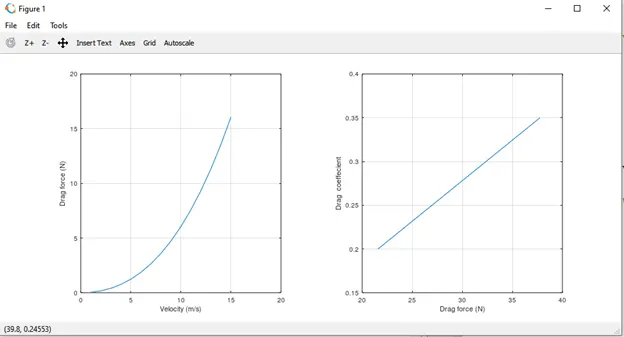
CONCLUSION :

• From plot between Velocity and Drag force, we can see that there is a non linear.

• From plot between Drag coefficient and Drag force, we can see that there is a linear relation in them, or in other words as the value of Drag coefficient decreases, the value of Drag force also decreases linearly. That is due to our assumption of taking the velocity as constant and then varying the drag coefficient due to change in the area.

REFERENCES :

https://www.researchgate.net/publication/331366310_CFD_analysis_of_an_exceptional_cyclist_sprint_position

https://link.springer.com/article/10.1007/s12283-017-0234-1#Bib1