MATLAB program to perform Curve Fitting

Objective: To write a MATLAB program to perform Curve Fitting

Theory:

Curve fitting is the process of constructing a curve or mathematical function, that has the best fit to a series of data points, possibly subject to constraints. Curve fitting can involve either interpolation, where an exact fit to the data is required, or smoothing, in which a "smooth" function is constructed that approximately fits the original data. This can also help in visualizing the level of uncertainty present in the curve. Fitted curves can be used as an aid for data visualization, to infer values of a function where no data are available, and to summarize the relationships among two or more variables.

Curve fitting serves as an important tool in analyzing the forecast of any trends from the past data Eg; Population growth.

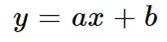
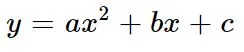
Polynomials, Quadratics, Cubic, Straight Lines are the most convenient Equations to perform Curve fitting.

• Straight-line

• Quadratic Equation

• Cubic Equation

How to make a curve fit perfectly?

• A perfect Curve fit refers to that curve which mathematically represents the original data set, independent of the degree of the polynomial equation. How to get the best fit?
• The best fit Comes with no error/zero error after considering the values of the entire dataset.
• The best fit line can be calculated by minimizing the distance between the actual output and the predicted output. There are several methods to do this like sum of squared errors, the sum of absolute errors, root mean squared error, etc.
• Difference between the predicted output and the actual output should be the least.

Example:

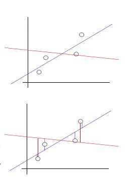
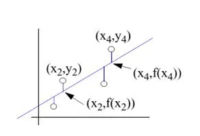
The above figure contains 4 values in its dataset and a curve fitting is performed,

• A blue line appears to be the best fit compared to the Redline because of the summation of error ie; the distance between the data points and the fitted blue line is less compared to Redline.
• The curve which gives the minimum possible error is termed as the best fit.

One such method of arriving at the best fit by minimizing error is Least Square Approach Method

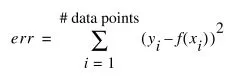
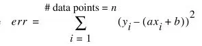
Once the curves are fitted to a dataset, the goodness of the can be evaluated using the following techniques,

1. Sum of Squares due to Errors (SSE)
2. R-Square
3. Adjusted R-Square
4. Root Mean Squared Error (RMS)

• Sum of Square due to Error

SSE is simply the summation of the Standard Deviations. Lower the SSE, the fit is considered to be Best.

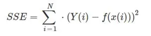
Finding an error in SSE can be related to the example shown in the least Square Approach.

• R-Square

It is the square of the correlation between the response values and the predicted response values. The higher the value of R-Square better will be the fit.

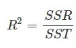Where,

SSR = Sum of Squares of Regression

SST = SSR + SSE

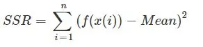
The R-Square value ranges from 0 to 1. R-Square value 1 indicated that the fit has been considered across 100% variation on the dataset from the Mean Average.

R-Squared is a statistical measure of fit that indicates how much variation of a dependent variable is explained by the independent variable(s) in a regression model.

• Adjusted R-Square

R-Squared only works as intended in a simple linear regression model with one explanatory variable. With a multiple regression made up of several independent variables, the R-Squared must be adjusted. The adjusted R-squared compares the descriptive power of regression models that include diverse numbers of predictors. Adjusted R-Square considers adding variables that are completely independent, but still related to the system in an infinitely small manner.

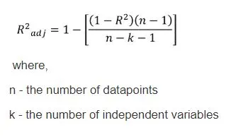
• Root Mean Squared Error

RMS is the standard deviation of the residuals (prediction errors). Residuals are a measure of how far from the regression line data points are; RMSE is a measure of how to spread out these residuals are. In other words, it tells you how concentrated the data is around the line of best fit.

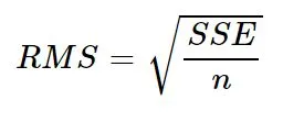
"n" refers to the number of points in the dataset.

The data used in this program contains 3200 values of Specific Heat of Oxygen at different Temperatures.

The goodness of the Fits is evaluated in this program by considering R-Square and RMS values.

code to plot linear and cubic fit:

clear all
close all
clc

% to load the dataset file
cp_data=load('data');

%preparing the data
temperature=cp_data(:,1);
cp=cp_data(:,2);
mean_cp=mean(cp);
n=3200;

%curve fit

%linear fit
co_eff1=polyfit(temperature,cp,1);
predicted_cp1=polyval(co_eff1,temperature);


figure(1)
hold on
plot(temperature,cp,'linewidth',2,'color','r')
plot(temperature,predicted_cp1,'linewidth',2,'color','b')
xlabel('temperature [K]');
ylabel('Specific Heat [KJ/Kmol-K]');
legend('Original Data','Linear fit','location','NorthWest');
axis([0 4000 800 1500]);

error_1=cp-predicted_cp1;
sse_1=sum(error_1.^2);
ssr_1=sum((cp-mean_cp).^2);
sst_1=sse_1+ssr_1;
rsquare_1=ssr_1/sst_1
rms_1=sqrt(sse_1/n)

%Quadratic fit
co_eff2=polyfit(temperature,cp,2);
predicted_cp2=polyval(co_eff2,temperature);

figure(2)
hold on
plot(temperature,cp,'linewidth',2,'color','r')
plot(temperature,predicted_cp2,'linewidth',2,'color','b')
xlabel('temperature [K]');
ylabel('Specific Heat [KJ/Kmol-K]');
legend('Original Data','quadratic fit','location','NorthWest');
axis([0 4000 800 1500]);

error_2=cp-predicted_cp2;
sse_2=sum(error_2.^2);
ssr_2=sum((cp-mean_cp).^2);
sst_2=sse_2+ssr_2;
rsquare_2=ssr_2/sst_2
rms_2=sqrt(sse_2/n)

%Cubic fit
co_eff3=polyfit(temperature,cp,3);
predicted_cp3=polyval(co_eff3,temperature);

figure(3)
hold on
plot(temperature,cp,'linewidth',2,'color','r')
plot(temperature,predicted_cp3,'linewidth',2,'color','b')
xlabel('temperature [K]');
ylabel('Specific Heat [KJ/Kmol-K]');
legend('Original Data','cubic fit','location','NorthWest');
axis([0 4000 800 1500]);

error_3=cp-predicted_cp3;
sse_3=sum(error_3.^2);
ssr_3=sum((cp-mean_cp).^2);
sst_3=sse_3+ssr_3;
rsquare_3=ssr_3/sst_3
rms_3=sqrt(sse_3/n)

%Poly fit
co_eff4=polyfit(temperature,cp,4);
predicted_cp4=polyval(co_eff4,temperature);

figure(4)
hold on
plot(temperature,cp,'linewidth',2,'color','r')
plot(temperature,predicted_cp4,'linewidth',2,'color','b')
title('4th order polynomial')
xlabel('temperature [K]');
ylabel('Specific Heat [KJ/Kmol-K]');
legend('Original Data','polynomial fit','location','NorthWest');
axis([0 4000 800 1500]);

error_4=cp-predicted_cp4;
sse_4=sum(error_4.^2);
ssr_4=sum((cp-mean_cp).^2);
sst_4=sse_4+ssr_4;
rsquare_4=ssr_4/sst_4
rms_4=sqrt(sse_4/n)

%Poly fit
co_eff5=polyfit(temperature,cp,5);
predicted_cp5=polyval(co_eff5,temperature);

figure(5)
hold on
plot(temperature,cp,'linewidth',2,'color','r')
plot(temperature,predicted_cp5,'linewidth',2,'color','b')
title('5th order polynomial')
xlabel('temperature [K]');
ylabel('Specific Heat [KJ/Kmol-K]');
legend('Original Data','polynomial fit','location','NorthWest');
axis([0 4000 800 1500]);

error_5=cp-predicted_cp5;
sse_5=sum(error_5.^2);
ssr_5=sum((cp-mean_cp).^2);
sst_5=sse_5+ssr_5;
rsquare_5=ssr_5/sst_5
rms_5=sqrt(sse_5/n)

Code Explanation:

Terms:

polyfit here you put in (x-coordinate, y-coordinate, N) and it gives you coefficients. This command is used to generate the coefficients of the equations where temperature and cp values are variables.

polyvalent It uses coefficient and data points to find an output. this command is used to get the predicted cp values with the generated coefficients against the same temperature range.

the load command is used to loads the dataset from the current folder.

data: 1st column is temperature and 2nd column is cp values.

mean command is used to calculate the average of the cp values.

plot commands are used to plot the curves cp, predicted _cp against temperature.

hold on avoids the overwriting of plots.

linewidth & color defines the geometry of curves.

labeling of the axis is given by xlabel & ylabel.

legend helps to differentiate the curves, and the location is used to place the legend.

axis is used to constrain the graph limits.

error_x, sse_x, ssr_x, sst_x, rsquare_x, rms_x are the formulas to evaluate the goodness of fit as explained in the theoretical sect00ion.

Stepwise explanation

1. We have to assign the value of temperature and C_p from the datasheet.cp .we then calculate the mean C_p. We find the value of the coefficient of a polynomial with help of polyfit command.
2. Using polyfit command find the coefficients of the polynomial.
3. Using these coefficients and temperature data find the value of predicted C_p
4. Plot the graph for the Temperature vs C_p and Temperature vs predicated C_p. the difference in value of C_p in the graph is shown with help of legend command.
5. To check the goodness of the curve we have entered the above equations for the sum of squares due to error (SSE), R-square, Adjusted R-square, Root mean squared error (RMSE) in the above code
6. To find the errors, we have used FOR LOOP, to find the total value of SSE and SSR first we have found the SSR and SSE for each value of cp using FOR LOOP, and SSE and SSR for each value are named as ‘x’ and ‘y’ respectively and their formula is defined.
7. Now after the FOR LOOP is executed total SSE and SSR are calculated by adding the values of ‘x’ and ‘y’ buy using ‘sum()’ command.
8. After entering the above equations and running the code we will get the value of these terms in the workspace or in the command window.
9. we can see the values of the sum of squares due to error (SSE), R-square, Adjusted R-square, Root mean squared error (RMSE). Here value of R-square is 0.9249 which is considered not to be good and the value of RSME is also very large that means the data points very far away from the curve fit. So by increasing the order of the polynomial, we can obtain good value of these quantities.

Plots and Results:

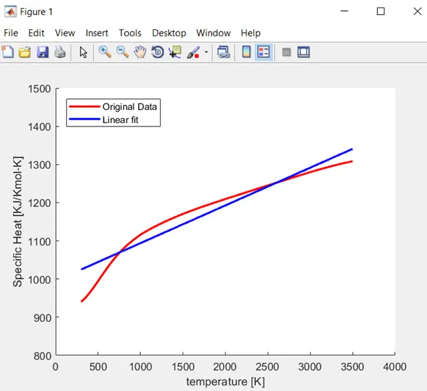
fig:Linear fit

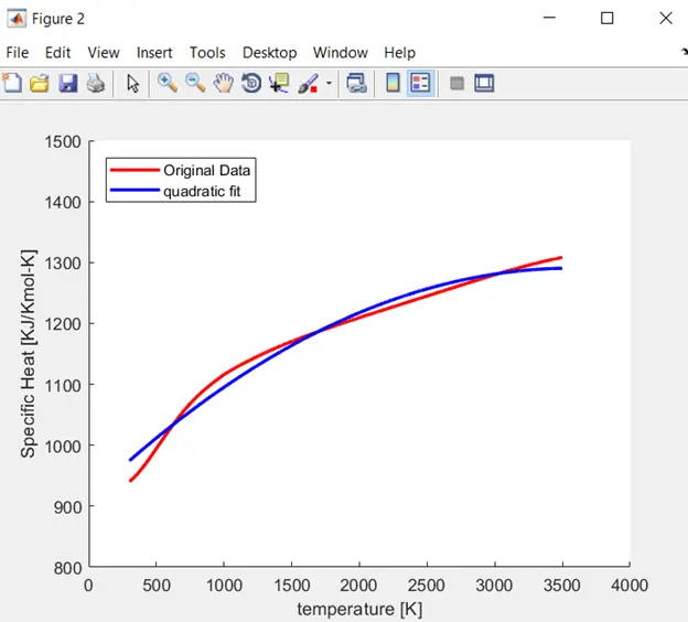
fig:Quadratic fit

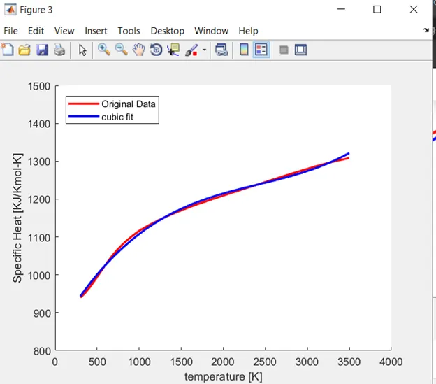
fig:Cubic fit

Discussion

From the above results it can be clarified that by increasing the order of the polynomial, a best fit can be obtained.

The Best fit should have an R-Square value ranging from 0.95 to 1, where in this case Cubic fit (R-Square =0.99) is the Best fit.

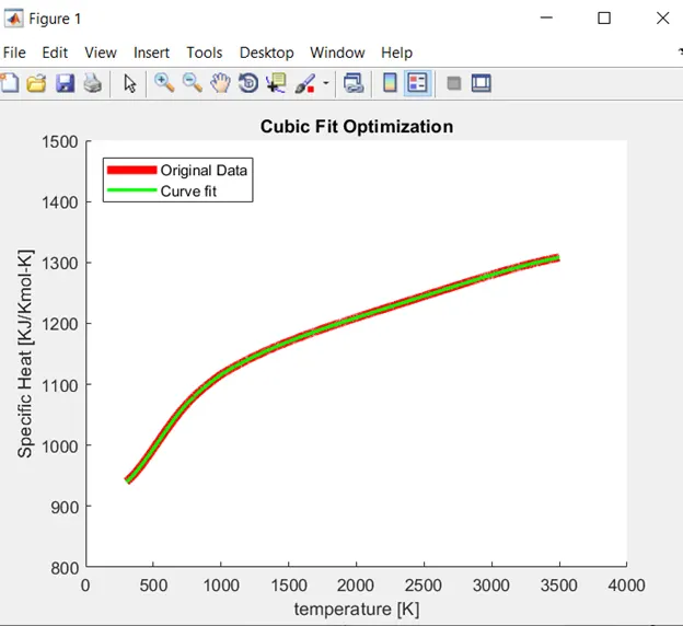
Fits can still be optimized by increasing the order of polynomial equation as shown below,

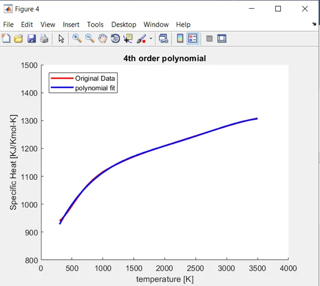
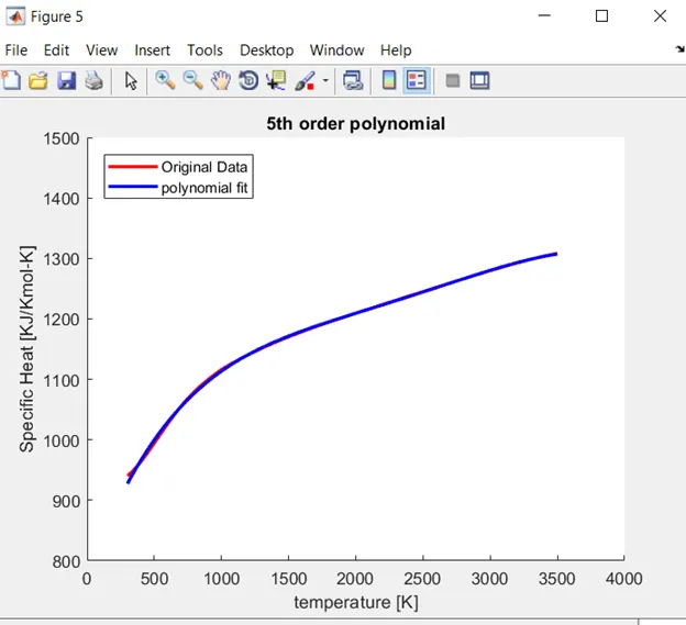
• Could be done to improve the Cubic Fit

To improve the Cubic Fit is to split the existing data set into 2 or more sets, according to feasibility.

Once the data set is split, use polyfit and polyval commands to each dataset and then plot the curves.

code for split operation:

clear all
close all
clc

% to load the dataset file
cp_data=load('data');

%preparing the data
temperature=cp_data(:,1);
cp=cp_data(:,2);
mean_cp=mean(cp);
n=3200;

%splitting the dataset

temperature_1=cp_data(1:500,1);
cp_1=cp_data(1:500,2);

temperature_2=cp_data(501:800,1);
cp_2=cp_data(501:800,2);

temperature_3=cp_data(801:1200,1);
cp_3=cp_data(801:1200,2);

temperature_4=cp_data(1201:1600,1);
cp_4=cp_data(1201:1600,2);

temperature_5=cp_data(1601:2500,1);
cp_5=cp_data(1601:2500,2);

temperature_6=cp_data(2501:3200,1);
cp_6=cp_data(2501:3200,2);

%curve fit

co_eff1=polyfit(temperature_1,cp_1,3);
predicted_cp1=polyval(co_eff1,temperature_1);

co_eff2=polyfit(temperature_2,cp_2,3);
predicted_cp2=polyval(co_eff2,temperature_2);

co_eff3=polyfit(temperature_3,cp_3,3);
predicted_cp3=polyval(co_eff3,temperature_3);

co_eff4=polyfit(temperature_4,cp_4,3);
predicted_cp4=polyval(co_eff4,temperature_4);

co_eff5=polyfit(temperature_5,cp_5,3);
predicted_cp5=polyval(co_eff5,temperature_5);

co_eff6=polyfit(temperature_6,cp_6,3);
predicted_cp6=polyval(co_eff6,temperature_6);


figure(1)
hold on
plot(temperature,cp,'linewidth',5,'color','r')
plot(temperature_1,predicted_cp1,'linewidth',2,'color','g')
plot(temperature_2,predicted_cp2,'linewidth',2,'color','g')
plot(temperature_3,predicted_cp3,'linewidth',2,'color','g')
plot(temperature_4,predicted_cp4,'linewidth',2,'color','g')
plot(temperature_5,predicted_cp5,'linewidth',2,'color','g')
plot(temperature_6,predicted_cp6,'linewidth',2,'color','g')
title('Cubic Fit Optimization');
xlabel('temperature [K]');
ylabel('Specific Heat [KJ/Kmol-K]');
legend('Original Data','Curve fit','location','NorthWest');
axis([0 4000 800 1500]);

On performing split operation, cubic fit has managed to trace the original data set.

Comparison of the goodness of fit for various degree of the polynomial

Curve fit toolbox is an inbuilt app in the MATLAB. In this app, we have to give some input data and it generates the curve fit automatically and it is also giving the value of SSE, R-square, Adjusted R-square, and RMSE.

For our data, here is the screenshot of linear and cubic fit of curve fit toolbox respectively

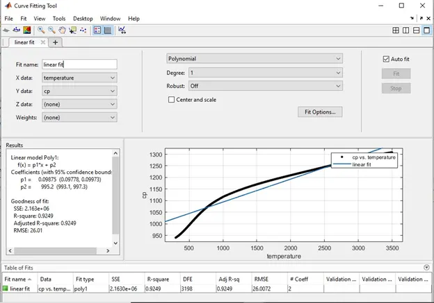
fig:Linear fit

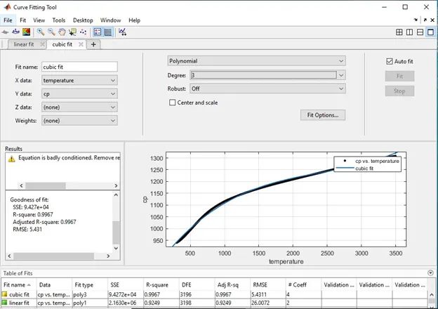
fig:Cubic fit

The value of R-square is 1 for the 8^th order of the polynomial. Below is the 8^th order of polynomial curve fit.

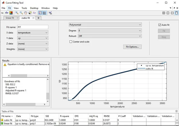
fig:Perfect fit

To make a curve fit perfect

• A perfect Curve fit refers to that curve which mathematically represents the original data set, independent of the degree of the polynomial equation.
• To make a perfect fit, we must consider error estimates as well. Perfect fit means, the curve should fit the original curve without showing any errors (such as centering and scaling erros) in that particular degree of the polynomial.
• A perfect fit is a fit in which the value of R-square is 1. So, this is only possible when actual curve and predicated curve meet at all points. As I say above that I found that R-square value is 1 for the 8^thorder of the polynomial. So, by increasing the order of polynomial we make the curve perfectly fit.

Conclusion:

• There are many methods that can be used to make the cure fit properly.
• We need to have high order polynomial equations to achieve the best fit.
• By splitting the data we get a better fit, more the number of splits, the better the output results.

References

• Curve Fitting Basics: https://en.wikipedia.org/wiki/Curve_fitting
• Goodness of Fits: https://projects.skill-lync.com/projects/Curve-Fitting-and-criterion-to-choose-best-fit-41860