Breaking Ice with Air cushion Vehicle - Finding minimum pressure with Newton-Raphson method using Python

• problem statement:

For this challenge, writing a python script to solve for the minimum value of pressure using the newton raphson method.

where p denotes the cushion pressure, h the thickness of the ice field, r the size of the air cushion, σ the tensile strength of the ice and β is related to the width of the ice wedge.

Take β = 0.5, r = 40 feet and σ = 150 pounds per square inch (psi).

1. Use the newton raphson method to find out the value of pressure for h = 0.6 ft.

2. Find the optimal relaxation factor for this problem with the help of a suitable plot.

3. Tabulate the results of p for h = [0.6,1.2,1.8,2.4,3,3.6,4.2] assuming a suitable relaxation factor

• Aim:

Determining minimum pressure to break ice using an air cushion ice breaker - Newton Raphson method

• OBJECTIVE:

To determine the minimum cushion pressure needed to break a given thickness of ice

using an air cushion vehicle through Newton-Raphson method using Python.

To find an optimum relaxation factor in the case of breaking an ice wedge of thickness equal to 0.6 feet using Newton Raphson Method

• THEORY:

The Newton-Raphson method (also known as Newton's method) is a way to quickly find a good approximation for the root of a real-valued function f(x)=0. This method is based on linear approximation where it uses the idea that a continuous and differentiable function can be approximated by a straight line tangent to it.

Here is a picture to demosterate what Newton's method actudally does:

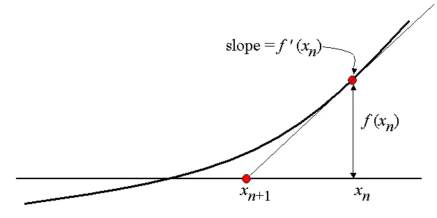
We draw a tangent line to the graph of f(x) at the point Both tangents are always intersected at the axis, except when they are in parallel (in such cases, root is not possible).

Equation to be solved:

To determine the minimum pressure Muller (“Ice Breaking with an Air Cushion Vehicle”) in Mathematical Modeling: Classroom Notes in Applied Mathematics, SIAM 1987) derived the equation

• Target Equation:

p3(1−β)+(0.4β2−(σh2r2))p2+σ2h43r4p−(σh23r2)3=0p3(1-β)+(0.4β2-(σh2r2))p2+σ2h43r4p-(σh23r2)3=0

1st order derivative:

f'(p)=3p2(1−β2)+(0.4hβ2−σha2r2)2p+σ2h43r4f′(p)=3p2(1-β2)+(0.4hβ2-σha2r2)2p+σ2h43r4

Newton-Raphson is performed using:

Pguess=Pguess+α(f(Pguess)f'(Pguess))Pguess=Pguess+α(f(Pguess)f′(Pguess))

Here p = cushion pressure

h = thickness of the ice field

r = size of the air cushion

σ = tensile strength of the ice

β = related to the width of the ice wedge.

import matplotlib.pyplot as plt
import math
import numpy as np

# Defining the function
def function(p,h):
	term1 =pow(p,3)*(1-pow(beta,2))
	term2 =(0.4*h*pow(beta,2) - sigma*pow(h,2)/pow(r,2))*pow(p,2)
	term3 =pow(sigma,2)*pow(h,4)*p/(3*pow(r,4))
	term4 =pow((sigma*pow(h,2))/(3*pow(r,2)),3)
	term = term1+term2+term3-term4
	return term

# Defining the derivative of the function
def function_prime(p,h):
	term5=3*pow(p,2)*(1-pow(beta,2))
	term6=(0.4*h*pow(beta,2) - sigma*pow(h,2)/pow(r,2))*2*p
	term7=pow(sigma,2)*pow(h,4)/(3*pow(r,4))
	term_r = term5+term6+term7
	return term_r

#Input
r = 40 #size of air
beta = 0.5 #width of ice wedge
sigma = 150 #tensile strength
height = [0.6,1.2,1.8,2.4,3.0,3.6,4.2] #thickness of ice field
p_guess = 50 #cushion pressure to start iteration
alpha = 1 #relaxation factor
tol = 1e-4 #tolerance
pressure = []

iter = 1 #number of iteration
for h in height:
	while(abs(function(p_guess,h))>tol):
		p_guess = p_guess- alpha*(function(p_guess,h)/function_prime(p_guess,h))		
		iter = iter + 1	
	pressure.append(p_guess) #storing values of pressure in pressure array

for i in range(0,7):
	if i == 0:
		print(" : height : pressure")
	print(" | ", height[i]," | ", pressure[i])

print("Number of iterations = ",iter,)
plt.plot(height,pressure)
plt.title('Cushion presuure Vs thickness of ice field')
plt.xlabel('thickness of ice field')
plt.ylabel('Pressure')
plt.show()

code explanation

frist of All the required modules are imported using import comand, math for mathematical functions, matplolib for plotting, numpy for array processing
Functions(p, h) and function_prime(p, h) are defined which are further used for calculating the value of the non-linear function and its first derivative at diffferent values of pressure 'p' and ice wedge thickness 'h' and 'return' command is used in both the functions to return the required outputs when the functions are called further in the program.
Input parameters are assigned as beta = 0.5, r = 40 feet, sigma = 150 pounds per square inch (psi) and h = [0.6, 1.2, 1.8, 2.4, 3.0, 3.6, 4.2] feet.
We are now assuming p_guess = 50(first guess value of pressure, relaxation factor i.e alpha = 1, tolerance = 1e-4 and i = 1.
pressure is created as empty arrays for storing the values.

For calculating minimum value of pressure, using Newton Raphson Method, for different values of ice wedge thickness 'h' a 'for' loop with a counter variable 'height' is defined and used. Inside a for loop, a while loop is used to obtain the minimum value of pressure with the condition that loop will run till the absolute value of function 'f(p, h)' for p_guess and a(thickness for particular iteration of for loop) i.e 'abs(f(p_guess, a))' is greater than the tolerance value i.e 'tol'. Syntax used is 'while (absf(p_guess, a)) > tol):'. An absolute value of function is used because sometimes it is possible that Newton Raphson Method must not converge solutions and may take many iterations to reach the actual value of a root of the function. Therefore, we need to take modulus of the function, since, if in case value of function is slightly negative, the value after taking modulus will be greater than the tolerance value i.e 'tol'. Inside the while loop, the modified equation of Newton Raphson Method is defined and also the value of a variable 'iter' is defined as equal to 'iter + 1' so that it gets updated.

Also, the arrays 'pressure' gets appended for every iteration of the 'for' loop. Which help to storing values of pressure in pressure array

A graph of ice wedge thickness versus minimum cushion pressure is plotted with the help of command 'plt.plot' and passing the arrays 'cushion_pressure' and 'number_of_iterations' as an input arguments.

output of case 1 :

import matplotlib.pyplot as plt
import math
import numpy as np

# Defining the function
def function(p,h):
	term1 =pow(p,3)*(1-pow(beta,2))
	term2 =(0.4*h*pow(beta,2) - sigma*pow(h,2)/pow(r,2))*pow(p,2)
	term3 =pow(sigma,2)*pow(h,4)*p/(3*pow(r,4))
	term4 =pow((sigma*pow(h,2))/(3*pow(r,2)),3)
	term = term1+term2+term3-term4
	return term

# Defining the derivative of the function
def function_prime(p,h):
	term5=3*pow(p,2)*(1-pow(beta,2))
	term6=(0.4*h*pow(beta,2) - sigma*pow(h,2)/pow(r,2))*2*p
	term7=pow(sigma,2)*pow(h,4)/(3*pow(r,4))
	term_r = term5+term6+term7
	return term_r
#Inputs
r = 40
beta = 0.5
sigma = 150
height = 0.6
p_guess = 50 
tol = 1e-4 
pressure = []

iter = 1
a1= []
itera= []
for a in range(1,200):
	a = a*0.01

	iter = 1
	p_guess = 50
	while (abs(function(p_guess,height)) > tol):
		p_guess = p_guess - a*(function(p_guess,height)/function_prime(p_guess,height))
		iter = iter + 1

	itera.append(iter)
	a1.append(a)
	print('relaxation factor=', p_guess)
	print('number of itration = ',iter)


plt.plot(a1,itera,color="green",linewidth=3)
plt.xlabel('relaxation factor',fontsize = 'large' , fontweight = 'bold')
plt.ylabel('No. of Iterations',fontsize = 'large' , fontweight = 'bold')
plt.title('relaxation factor vs No. of Iterations')
plt.savefig('alpha.png')
plt.show()

output of case 2 :