Basics of ML & AL Week 2 Challenge

Ans 1.

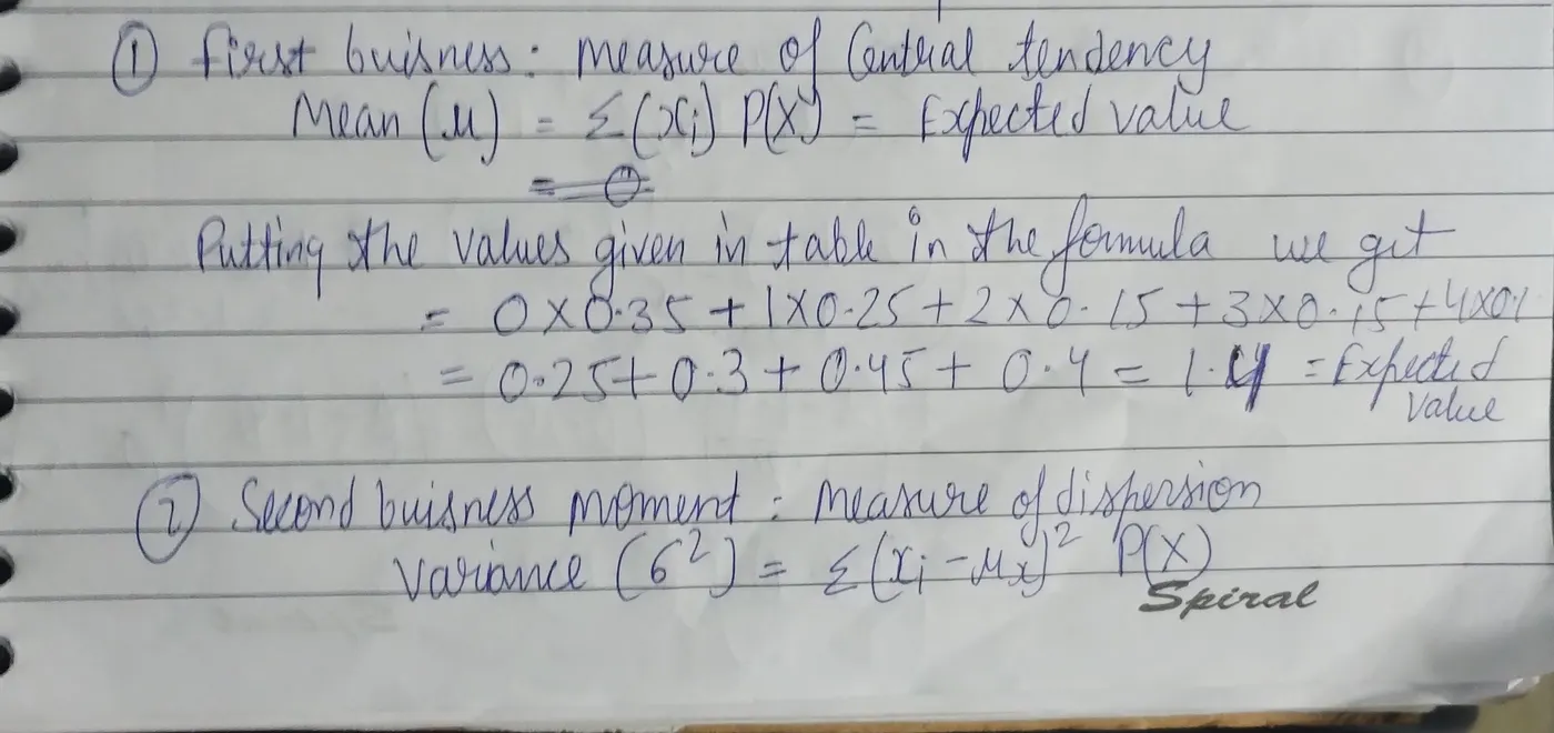
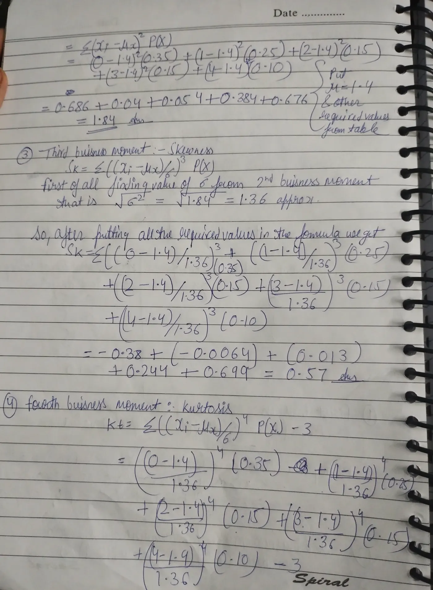
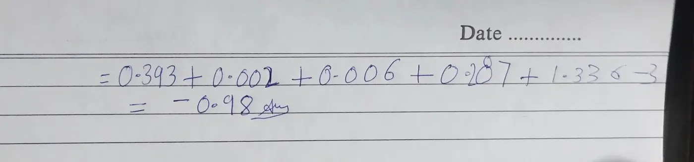
Ans 2) The expected value in statistics is a concept that provides insight into the long-run average outcome of a random variable based on its possible outcomes and their respective probabilities. The key differences between the expected value and the mean are:

1. Expected Value vs Mean:

• Expected Value: It represents the average result we would observe in the long run if an experiment (such as a game of chance) were repeated many times. Essentially, it's the weighted average of all possible outcomes, where each outcome's weight is its probability. The expected value is a predictive tool that helps us forecast likely outcomes in uncertain scenarios.
• Mean (Simple Average): The mean, also known as the arithmetic average, is calculated from raw data that is collected from the source. It is the sum of all of all observations divided by the number of observations. Unlike the expected value, which considers probabilities, the mean treats all observations equally.

2. Origin of expected value:

• The concept of expected value dates back to the 17th century when mathematicians Blaise Pascal and Pierre de Fermat correspond about gambling problems. They sought a rational way to divide stakes in a game interrupted before its conclusion. Expected value emerged from these early deliberations, providing a robust tool for predicting, strategizing, and optimizing decisions in uncertain situations.

3. Calculation of Expected Value:

• For a discrete random variable, which represents specific, distinct values (e.g., coin flips, dice rolls), the expected value is found by multiplying each possible value by its probability and summing these products.
• The Formula for the expected value of the discrete variable is:
• E(X) = Σ(x_i)(P(x_i)
• (X) is a random variable.
• (x_i) represents specific values.
• (P(x_i)) is the probability of x_i

4. Continous Probability Distributions:

• For continuous probability distributions, the expected value is simply the mean of the random variable. As sample sizes increase, sample averages converge to the expected value due to the law of large numbers.

In summary, while the simple mean provides an average based on observed data, the expected value offers a predictive lens for understanding long-term outcomes in uncertain scenarios. Both concepts play essential roles in statistics and decision-making.

Ans 3) Skewness in distribution refers to its asymmetry. When a distribution is right-skewed(also known as positive skew), it means that the tail on the right side of the peak is longer than the left side. Conversely, a left-skewed distribution (or negative skew) has a longer left tail. Here's what we need to know:

1. Zero skews: A distribution with zero skews is symmetrical, meaning its left and right sides are mirror images. Normal distributions have zero skews, but other symmetrical distributions (like uniform or some bimodal distributions) can also exhibit this property. In practice, real-world data often has a small amount of skew, but if it's close to being symmetrical, we consider it to have zero skew for practical purposes.

2. Right-Skewed(Positive Skew): A right-skewed distribution has a longer tail on the right side of its peak. Think of it as having more observations at the extreme right end, although they're relatively infrequent. An example is the number of sunspots observed per year, where a histogram shows a right-skewed distribution.

3. Interpreting Skewness:

• Moderate skew: if skewness is between -1 and -0.5 (negatively skewed) or between 0.5 and 1 (positively skewed), the data is moderately skewed.
• Highly Skewed: The data is highly skewed if skewness is less than -1(negatively skewed) or greater than 1 (positively skewed).
  

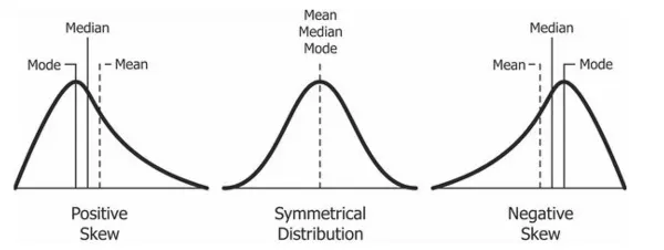
In statistical analysis, understanding skewness helps describe the distributions of variables and assess whether they adhere to assumptions (such as normality). While skewness itself isn't inherently "bad", it's essential to consider its implications based on the context of your analysis. Sometimes transformations (like log transformations) can be applied to mitigate skewness when necessary.

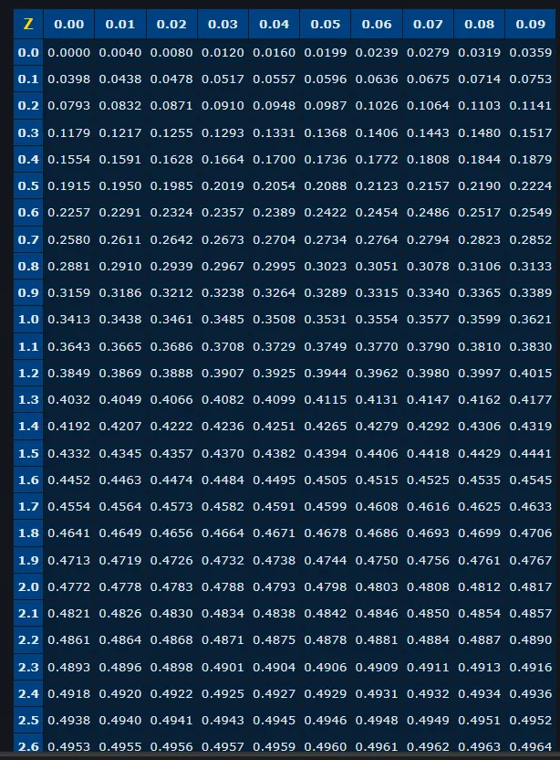
Ans 4) From the given data we have a value of mean= 680 and standard deviation =31 and the normal distribution table with Z-score value is given as follows:

So the required probability for the given data could be obtained as shown:

a) P(X<711)

Since we know for the continuous normal distribution Z- the score plays an important role and the formula for Z-score is (x-μ)/σ

so for X<711 ⇒ (X-680)/31<(711-680)/31 (substituting the given values of mean and std. deviation)

⇒ Z<1

From the above table, we can say, 0≤Z<1 = 0.3413 and Z< 0 = 0.5

So, Combining the above inequalities Z<1 ⇒ 0.5+0.3413= 0.8413

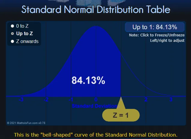
So, the required probability is 84.13%

b) P(X>740)

Calculating the Z value as shown For X>740,

(X-680)/31>(740-680)/31

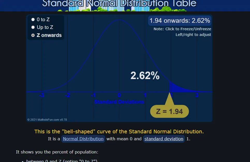
⇒Z>1.94

So, From the above table, We could say, the Z<0 value is 0.5 and for 0≤Z<1.94 value is 0.4732

so For Z>1.94 we could say value is 1-(0.5+0.4738)= 1-0.9738= 0.0262

So the required probability is 2.62%

C) P(600<X<760)

Calculating the Z value we get, (600-680)/31<Z<(760-680)/31

-2.58<Z<2.58, value is 0.4951X2= 0.9902

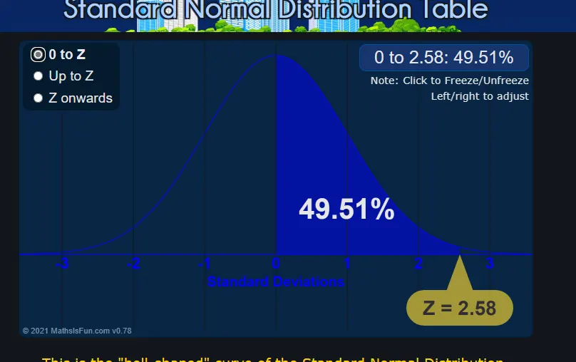
So the required probability is 99.02%.

D) P(X=720)

Since For X=720, the Value of Z is obtained as Z= (720-680)/31= This value of Z area in the normal distribution curve is 0 We could say probability, P(X=720)= 0%.

Ans 5) From the given data we have the curve as shown:

It's clear that the above curve shows the normal distribution of the data concerning varying values of random variable X, the whole graph shows the distribution of the population between 6 sigma (+3σ to -3σ ) values of random variable,

• The two dark blue areas with 34.1% values are distributed between 0 to σ and -σ to 0 each.
• The two Sky blue areas with 13.6 % values are distributed between -2σ to -σ and σ to 2σ each.
• The remaining two grey areas show values between -3σ to -2σ and 2σ to 3σ.
• So adding all of these values we get 99.7% values of data lying between the 3 standard deviation of the mean.
• 95% of data is within 2 standard deviations of the mean.
• 66% of the data is within 1 standard deviation of the mean.

This means that standard normal distributions make sure all the data following normal distribution have the same mean and standard deviation.