Assignment 7-Side Pole Crash Simulation Challenge

    I. OBJECTIVES

• To carry out the Side Pole Crash Analysis of a BIW for the given dummy car model.
• To set up the model as per the below-mentioned case and ensure the correct running of the simulation.
• To extract all the output requests and the mandatory results and document the whole procedure with proper explanations and conclusions.

• Side Pole Crash - BIW:

  1. Check unit system and either follow [Mg mm s] or [Kg mm ms].
  2. Create an appropriate interface, friction 0.2, and recommended parameters.
  3. Make sure of no penetrations and intersections.
  4. Create a rigid pole with friction 0.1 as per the reference model.
  5. Compare the model weight with the full-scale 300k nodes model and use added masses to reach the target weight of 700kg while getting CG about the required range.
  6. Initial velocity as shown in the picture.

  7. Add the following Output Requests:

     1. Sectional force in the cross member.
     2. The intrusion at B pillar, hinge pillar, and fuel tank region. Provide recommendations on what can help to reduce Fuel tank intrusion.
     3. Peak velocity of the inner node of the door. 
  8. Use a model checker to ensure good quality.
  9. Time-step :0.5 to 0.1 microseconds.
  10. Run 80 ms.

   II. GIVEN MODEL

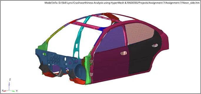Fig.1. Neon BIW model for Side Pole Crash

  III. PROCEDURE

1. The neon_side_reduced_0000.rad Starter file and the neon_front_0001.rad Engine file has been provided. For this project, we shall use both HyperMesh as well as HyperCrash for the set-up. 
2. The starter file is thus imported in HyperMesh via the Import Solver Deck. The model can be seen as shown in figure 1.

1. Frontal Crash - BIW

1. Check unit system and either follow [Mg mm s] or [Kg mm ms]

1. Once the model is imported, we can navigate to the BEGIN_CARD in the Cards subsection from the model tree. The Input Units would be visible which are set to [Kg mm ms] as seen in figure 2. Hence these are left unchanged. 

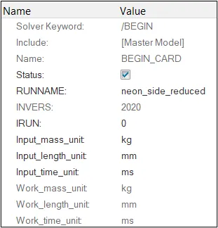
   Fig.2. Input Unit System

    

     2. Create an appropriate interface, friction 0.2, and recommended parameters

1. We start by removing the default interfaces and replacing them with our custom single Type 7 interface. Present interfaces are simply deleted by selection in the INTER subsection from the Solver Tree.
2. By right-clicking on the tree, we can select Create and navigate to INTER → Type 7. A new Interface card will be created which will be renamed as desired. 
3. All the nodes and elements are selected respectively to set the master and slave. The total number of each entity will be displayed.
4. As per the Friction of 0.2 and the recommended properties are concerned, the values are set as seen in figure 3.  

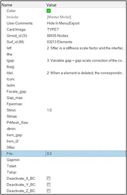
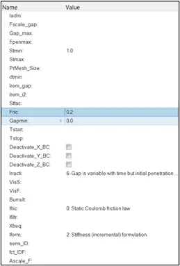
   Fig.3. Type 7 Interface with recommended properties

     3. Make sure of no penetrations and intersections 

1. The Penetration Check can be done by navigating to Tools → Penetration Check. 
2. Here the check type should be set to Intersections and penetrations. The selection type will be set to components where all the components are selected. 
3. The Check button is clicked. There was no kind of penetration present in the model.  

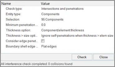
   Fig.4. Penetration Check

     4. Correct rigid bodies if any issues

1. No rigid body corrections were needed. 

     5. Create a rigid pole with the friction of 0.1

1. To create a Rigid Pole, we right-click on the Solver tree and navigate to RWall, and select CYL. A new card will get created and can be renamed,
2. An appropriate node is selected from the door section to get the reference coordinate for the pole. Figure 5 shows the selected node.  

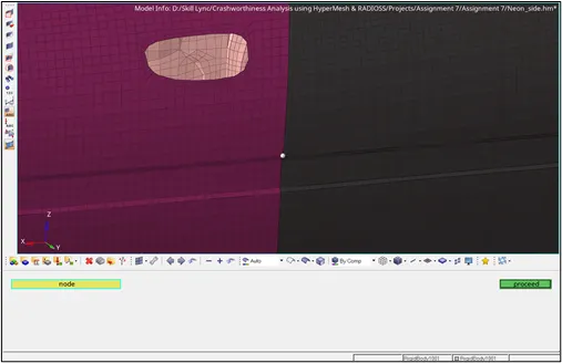
   Fig.5. Rigid Pole node placement

    
3. Since our body should be 5 to 10 mm away from the wall, the YM coordinate is changed accordingly. The Normal Z value is set as 1 to make the pole's side face against the car side. The Slide option is set to 2:Sliding with friction. With this, we can add our friction value as 0.1. The Dsearch value is set to 1000 and with this, the pole is created. 

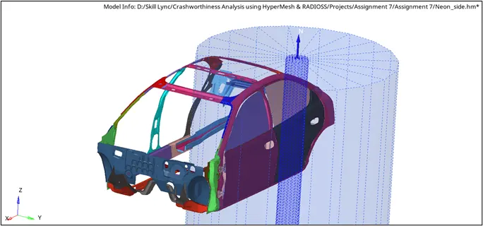
   Fig.6. Rigid Pole

     6. Compare the model weight with the full-scale 300k nodes model and use added masses to reach the target weight of 700kg while getting CG about the required range

1. The full model is opened in HyperCrash and is compared with the model we are working on. The COG of both the models lies on the same spot. Figures 7 and 8 show the CoG and Mass values as well as the point created to display the COG of our model. 

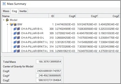
   Fig.7. Total Mass & CoG coordinates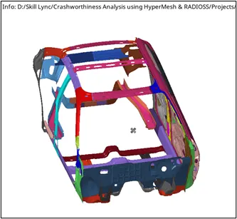

    

   Fig.8. Point of CoG

    
2. Our task is to get the total mass of the model up to 700 Kg and move the CoG towards the center in between the rails. The estimated addition of mass is approximately 533.693 kg. It can be seen that the current CoG lies more on the left due to some components. Hence, we distribute the mass in a 70:30 split with 373.585 Kg on the right and 160.1079 Kg on the left side. 
3. Now, the positioning of the mass addition and distribution has to be decided. We can assume that the seats will be mounted in a way that the mass will be distributed across the nodes in the area. We will create two mass additions, for left and right respectively.
4. To create the masses, we right-click on the Solver and navigate to Create and select ADMAS card. We create two such cards. 
5. Since we will be distributing the mass on every node we select, a general mass split can be done. As discussed, we put the respective masses on the left and the right rails.  

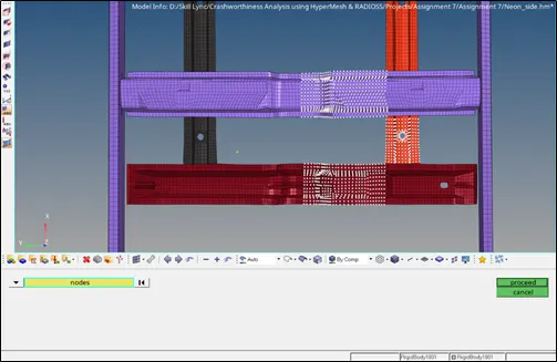
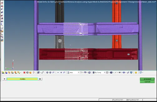
   Fig.9. Node selection for Mass Addition Distribution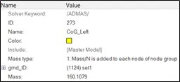

    

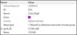
   Fig.10. Mass Addition Cards

    
6. Once the Mass addition is done, we can check the CoG and total mass from the Tools dropdown menu. We can achieve the final mass of 700 Kg. After plotting the coordinates of the CoG, we get the desired result. The following figures depict the same.

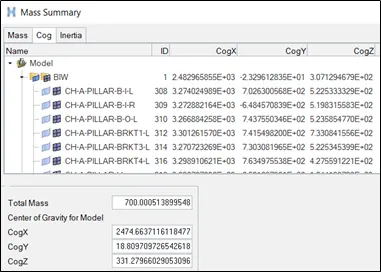
   Fig.11. Total Mass & final CoG coordinates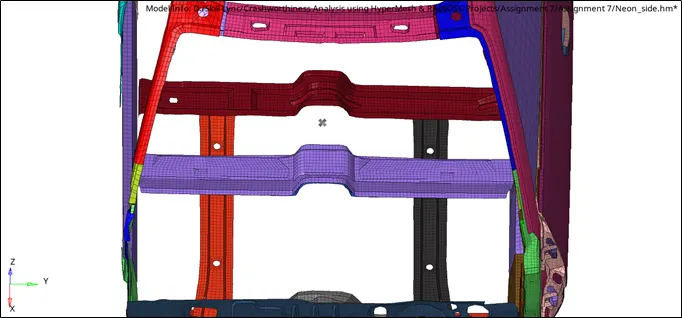

    

   Fig.12. The final point of CoG

     7. Initial velocity 35 mph 

1. The initial velocity is a boundary condition that is very straightforward to apply. We again right-click on the Solver tree and navigate to Create → BOUNDARY CONDITIONS → INIVEL. A new card under LOADS will be created. it is renamed accordingly.
2. Since the value of the initial velocity of 35 is given in mph, we will convert the units to mm/ms which comes out to be approximately 15.64 mm/ms. Thus, the velocity component will be [0,15.64,0] as our model will crash in the Y direction.

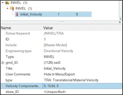
   Fig.13. Initial Velocity Card

     8. Adding the Output Requests

1. Before getting started with the Output requests, we have to add the sections for forces and intrusions.
2. Starting with the sections, we have to create 2 sections to get the forces on the middle rails. To create a section, we need a frame of reference that can act perpendicular to the area. Hence, by right-clicking on the Solver tree, we navigate to FRAME and select Mov, i.e. Moving frame. 
3. Now, the origin will be selected using the desired node selection. For the second reference, the option is toggled to the z-axis and a node is selected in the direction of the crash. The third reference node can be selected as desired. The create button is clicked and a frame with a local coordinate system is created as seen. 

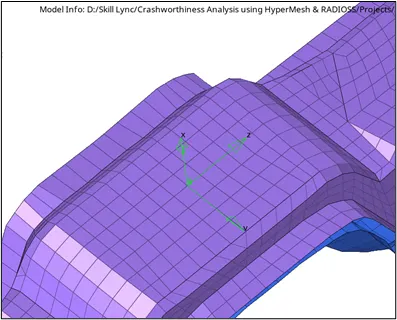
   Fig.14. Frame created

    
4. Once the frame is created, we can make the sections for the output requests. Again, by right-clicking on the Solver tree, we can navigate to SECT to create a section card. A total of 6 cards are created as discussed. Each one is renamed accordingly. 
5. Now, by clicking on the Frame_ID, we can select the respective frame system and create an infinite cross-sectional plane. 

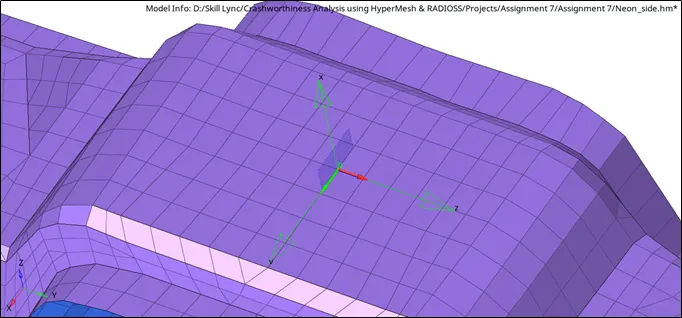
   Fig.15. Cross-section plane created

    
6. By right-clicking on grshel_id, we create a shell elements group. Clicking on Entity_id, we select two rows of elements to cover the area for output request.  

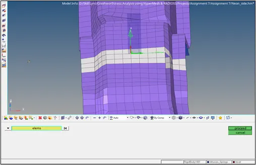
   Fig.16. Shell selection

    
7. This will finish the creation of one section. This shall be done for another one. Once created on their designated components, we can see them in figure 17. 

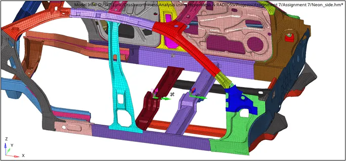
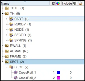
   Fig.17. All created Sections

     
8. To get the Intrusions, we will have to create Spring elements on the designated nodes. Spring elements are straightforward elements to create. The following three elements were created. 

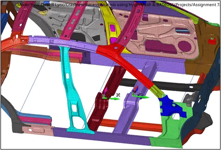
   Fig.18. Spring Elements for Intrusion

    
9. The Property card for the spring elements is created, and minimal values of mass and stiffness are given. The property is then assigned to the elements component. 

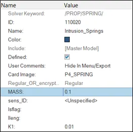
   Fig.19. Spring Elements Property card

    
10. For the Peak Velocity on the inner door node, we can create a new Output Block, rename it accordingly, and the Entity ID as 1 node that can be selected from the inner door component as seen in figure 20. Then the Variable for this node can be set to V: Translational Velocity (VX VY VZ).  

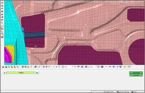
    Fig.20. Node selection for Peak Velocity Output Block

     
11. Now we move on to create the output requests from the above entities. For this, we use the output Block in the Model tree window. We create Output Blocks for the required number of results. The selection of the entities is done based on their types, i.e. sections, groups, etc. The following output blocks are created. 

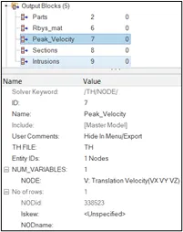
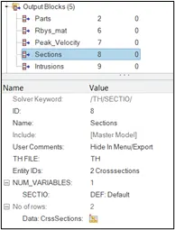
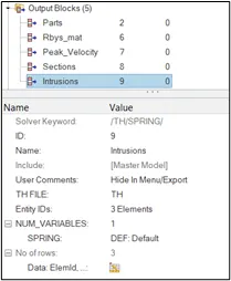
    Fig.21. Output Blocks

     9. Use a model checker to ensure good quality

1. To use the Model Checker, we navigate to the Model Checker in the Tools dropdown menu and select Radios Block. 
2. Once the Model Checker window is opened, the Run check option is clicked. When the checks are done, all the errors (if any) and the warnings will be displayed. As seen in figure 22, no errors were found. Though some warnings are displayed, they can be ignored since no major hindrance is caused by these warnings.

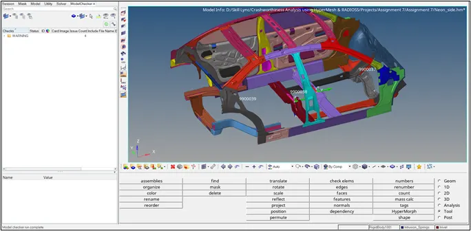
   Fig.22. Model Checker Results

    10. Time-step: 0.5 to 0.1 microseconds

1. To add the timestep, we change the value of Tfreq from the ENG_ANIM_DT to 5. 

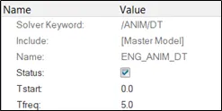
   Fig.23. Timestep Card

    11. Run 80 ms

1.  To run the model at 80 ms, we change the value of Tstop from the ENG_RUN to 80. 

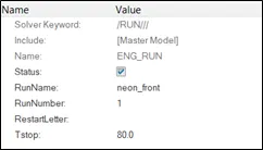
   Fig.24. Run Card

    
2. Now we can finally go to Analysis → RADIOSS → Save file as... → Rename file →  Radioss. The solver view will open and the simulation will start.

   IV. RESULTS

• After the simulation run is over, we get the following elapsed time and number of cycles: 

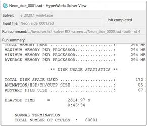
  Fig.25. Solver View Window

   
• Energy and Mass Error: 

  Fig.26. Output File Errors

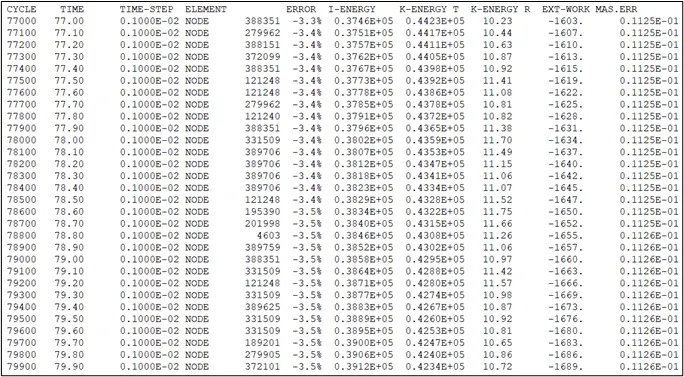
  It is clear from the Output file results that the value of the energy error lies between -15% and 5%. Also, the mass error does not exceed 1 which marks it workable.
• Crash Simulation Animations  To create the animations, we use the HyperView tool. The .h3d file from the simulation is extracted and then applied to play the animation. The animation helps us determine how the car's front structure reacts to the crash and how it deforms while dissipating energy.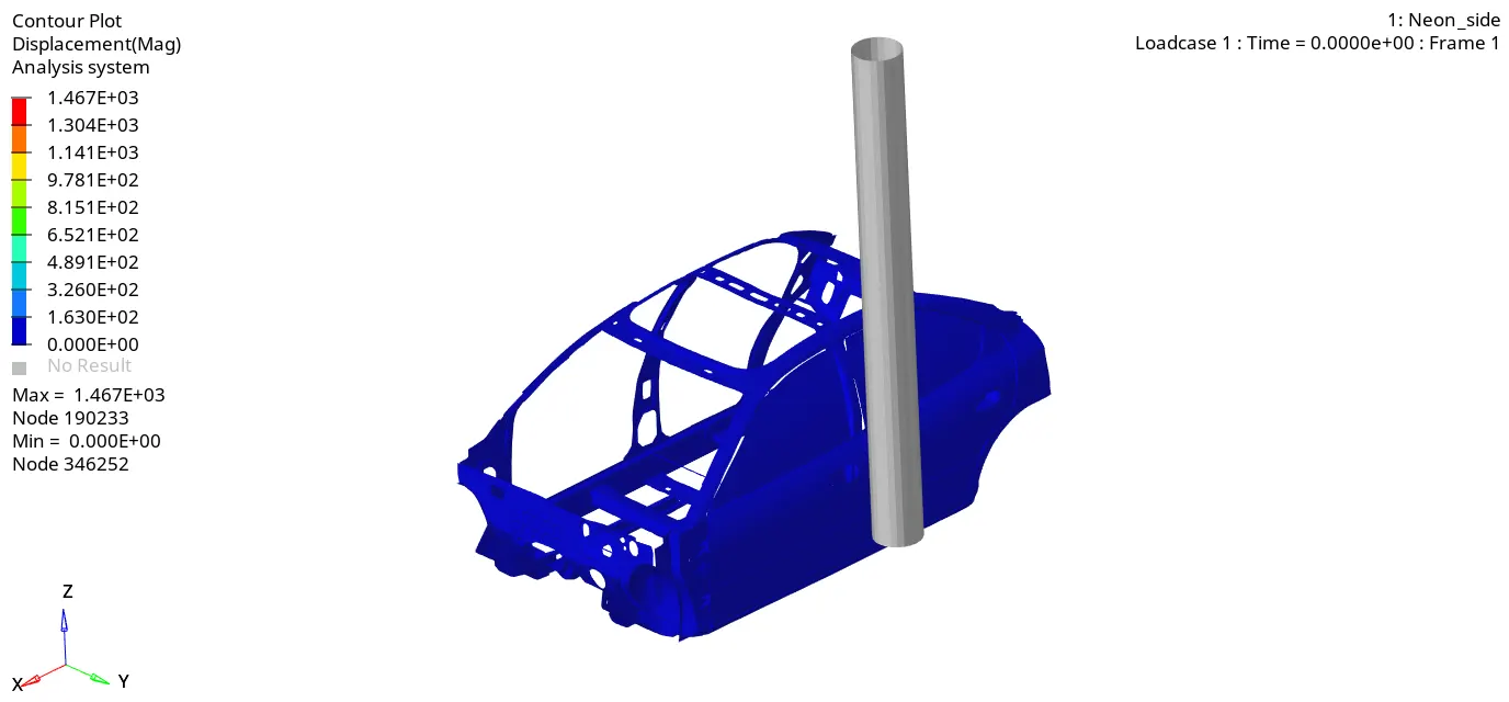  

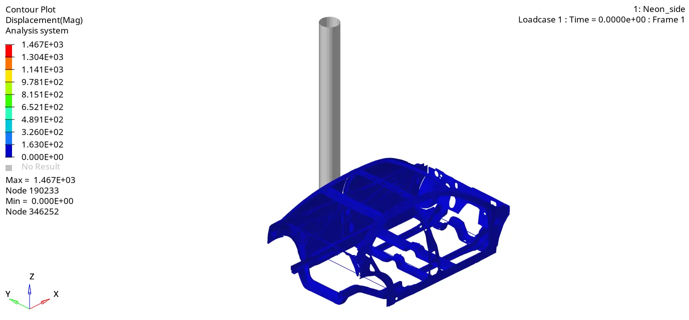
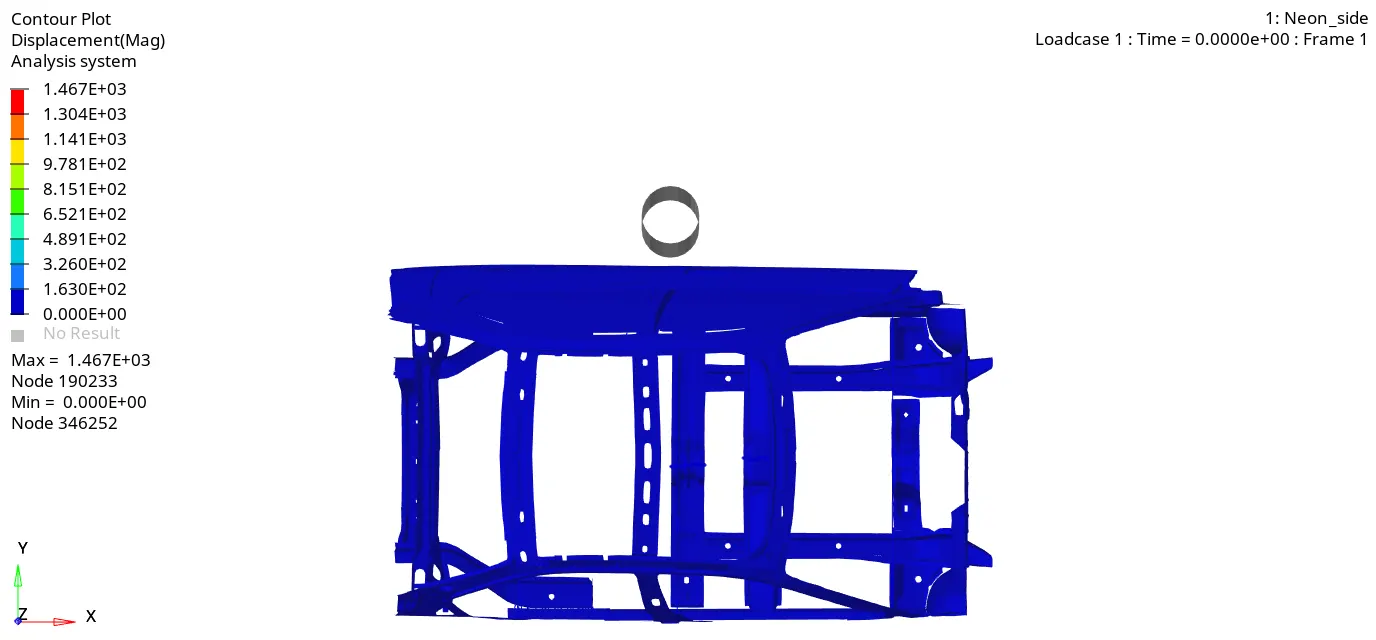
  Fig.27. Crash Animation with necessary views

   
• Result Graph Plots To plot the graphs from the results extracted from the simulation, we use the HyperGraph 2D tool. The T01 file is opened via this tool and the required graphs are plotted by selecting the Y-axis components.  ⇨ Energies Plot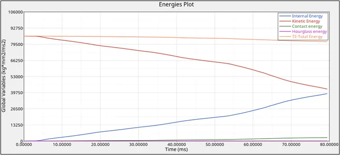 

  Fig.28. Energies Plot for Crash

  Here, five kinds of energies are plotted, namely, Internal, Kinetic, Contact, Hourglass, and Total Energy. The graph shows the energy characteristics resulting due to the behavior of the Car BIW during a side pole crash. For the first few milliseconds, there seems to be not much change since there is no contact. Once the body starts to crash into the wall, the internal energy starts to increase since stresses are generated inside the structure resulting in deformation. Understandably, the Kinetic energy decreases due to the decreasing velocity of the structure. All in all, the Total energy is almost constant, but due to the presence of slight Contact energy, the resultant value drops as well. Contact Energy is the energy applied by the system to avoid penetration of elements. After deformation occurs, the system will need to gradually apply more and more energy to avoid penetration of elements. We also avoided Hourglass energy by using the reduced integrated QEPH elements.   ⇨ Sectional Force in the Cross members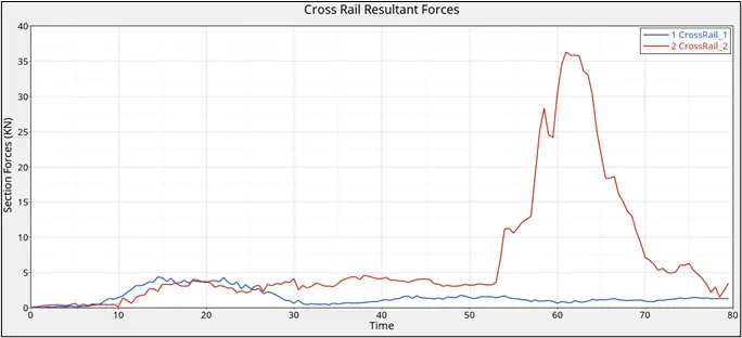

  Fig.29. Resultant Force Plot for Cross Rail Sections

  From the above plot, we can derive the max force values. The maximum force value on Front Rail was 4.33 KN and on Central Rail was 36.26 KN. The curve characteristics are different for both the rail sections. Since the central rail deforms more than the front rail due to its position, we get a spike in the force. This can be verified via crash animations.
  
  ⇨ Intrusions on the Pillars and Fuel Tank region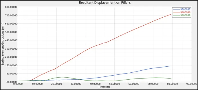

  Fig.30. Intrusion Displacement Plot on Pillars

  From the above plot, we can derive the elongation/displacement values. The maximum elongation on the hinge pillar spring element (9900037) was 162.15 mm, on the fuel tank region spring element (9900039) was 40.965 mm, and the highest value was seen on the B-Pillar spring element (9900038) which was 720.32 mm. A lower value is mandatory since passengers are to be kept harmless at the time of a crash. Also, from the animation, it can be verified that how the pillars elongate to ensure the passengers' safety. As far as the recommendation for the fuel tank intrusion is concerned, this region has the lowest intrusion of all, and also the test is done is at a high velocity. Even then the intrusion is not more than 4 cm. Hence, no recommendation is necessary. ⇨ Peak Velocity of the Inner Node of the Door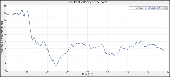

  Fig.31. Resultant Velocity Plot for the Inner Node

  From the above plot, we can derive the peak velocity value. The maximum velocity on the inner door node was found to be 17.04 mm/ms. This is due to the initial velocity we had given. When the impact occurs, the high characteristics of vibrations cause the velocity to peak even more. But once the deformation of the components takes place, the velocity starts decreasing. This goes to show that apart from absorbing the impact energy, dissipation of the vibrations from the collision is also important.
   

     V. CONCLUSIONS

• The following conclusion points can be drawn from the above assignment:-

1. The Side Pole Crash simulation of the Dodge Neon BIW was successfully carried out.
2. The model was properly set up for a successful simulation run without any errors.
3. Various Output Requests were created from the simulation to get the mandatory results. 
4. The behavior of the car structure was studied based on the results extracted from the simulation.