Assignment 7-Side Pole Crash Simulation Challenge

AIM:

To run a simulation for the Neon Side Pole Crash and to obtain the results in the post processing.

OBJECTIVE:

• To check the unit system in the solver.
• To create an appropriate interface with friction 0.2 and recommended parameters.
• To check for the penetrations and intersections in the component.
• To create cylindrical rigid wall with a friction 0.1.
• To add extra mass to attain a target mass of 700 kg.
• To apply initial velocity to the car.
• Keep the min time step of 0.1micro sec & max of 0.5micro sec.
• Run the model up to 80 milliseconds.
• To find the sectional force in the Cross member.
• To calculate the intrusions at the B-pillar, Hinge pillar and at Fuel tank region.
• To calculate the peak velocity of an inner node of the door.
• To request TH for all the inputs created.
• To run the simulation.
• To plot the graphs in the post processing.

THEORY AND INTRODUCTION:

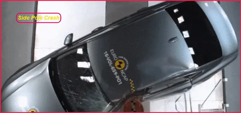
A side collision is a vehicle crash where the side of one or more vehicles is impacted. These crashes typically occur at intersections and in parking lots, and when two vehicles pass on a multi-lane roadway.

In the side pole impact collision cases, When the car gets crashes to the pole the load goes transferred to the car. So because of the load, it starts to deform and its contact with the dummy pelvis location. Pelvis position and orientation are important aspects of a vehicle occupant’s posture. Measurements of drivers’ or passengers’ pelvis locations are used for ergonomic or crash safety studies such as the development of posture prediction models, analysis of lap belt fit, and
development of computational human models.

Due to this structure to pelvis contact, the load has transferred to the occupant. As only a very small crumble zone is available during a side pole impact, so we have to ensure that the impact forces are distributed over a wide area. The B-Pillars and side members along the flanks of the vehicle are mainly responsible for this.

The impact forces are transferred from B Pillar to the opposite side of the vehicle first and foremost via the transversely rigid seat and the center console. A further load dissipation path runs from the base of the B pillar to cross member under the seat and transmission tunnel braces.

As per baseline study, identified the important load transfer path members are B-Pillar and its reinforcements, Roof bows, Sill, Transfers cross members. These parts stiffness increased by the way of design changes and material grade up.

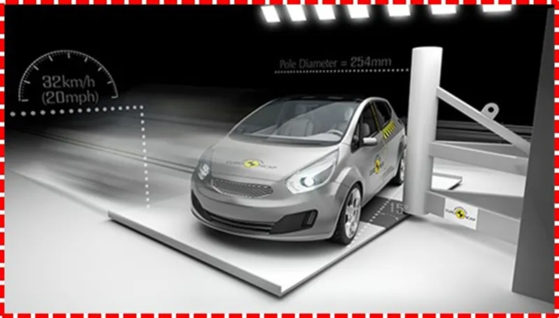
In this test, we are going to give the velocity to be 24 km/h and we are going to take the diameter of the pole to be 254 mm as the standard diameter value according to the FMVSS 214 standards.

PROCEDURE:

Phase 1-Check unit system and either follow [Mg mm s] or [Kg mm ms].

While opening hypermesh software,A user profile window will pop up,Switch to the radioss user profile as shown in below Figure 3 and start importing the model into the solver.

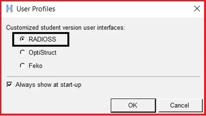
Now after switch the user profile to radioss,import the model (starter file) into the radioss solver deck.

To import the model,Go to Standard Panel >> Import >> Import Solver Deck.

Import Solver Deck option should be selected to import the radioss starter file.

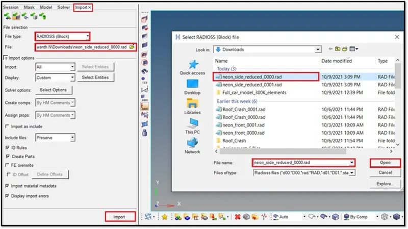
Here the import browser will appear as shown in above Figure 5,Select the appropriate starter file to import into GUI.

Switch the File Type to Radioss Block and import the model into GUI.Which is shown in below

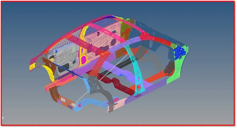
Here the model is in wireframe mode,Switch to the shaded mode as shown in below.

To switch to shaded mode,Go to Visualization Tab >> Shaded Elements and Mesh Lines.

Now go and check for the unit system of the model,To check for the unit system,Go to the Model Browser >> Control Cards >> BEGIN_CARD.

Check for the unit system is shown in below

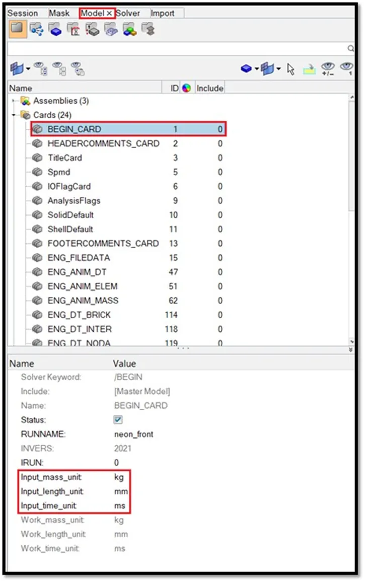
Now go to the HyperCrash,To go,Go to Menu Bar >> Applications >> HyperCrash.Which is shown in below.

Make sure whether the unit system in hypercrash is [ kN, kg, mm, ms].Which is shown

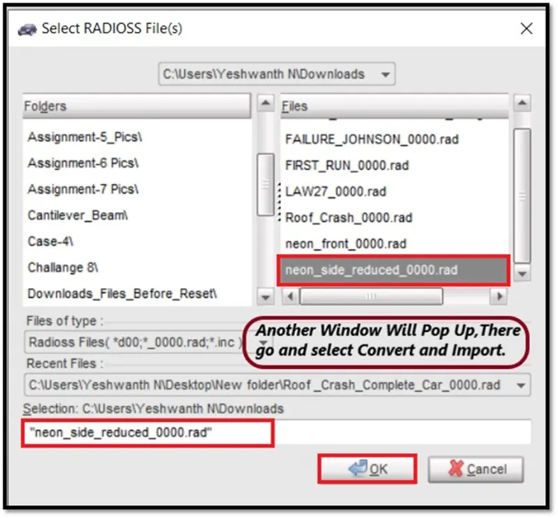
Now import the model in hypercrash,To import the model,Go to Menu Bar >> File >> Import >> Radioss.

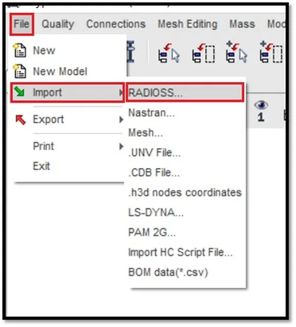
Here select the appropriate Radioss File and import the model into hypercrash.

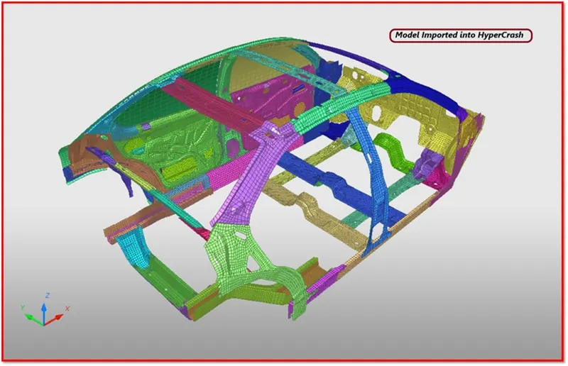
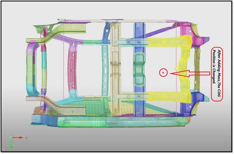
Here the COG is not in a proper position which is shown in below Figure 18.So we need add mass to get COG at proper position,Its like balancing.

To Check the Mass and COG [Centre of Gravity],Go to HyperCrash Menu Bar >> Mass >> Balancing,

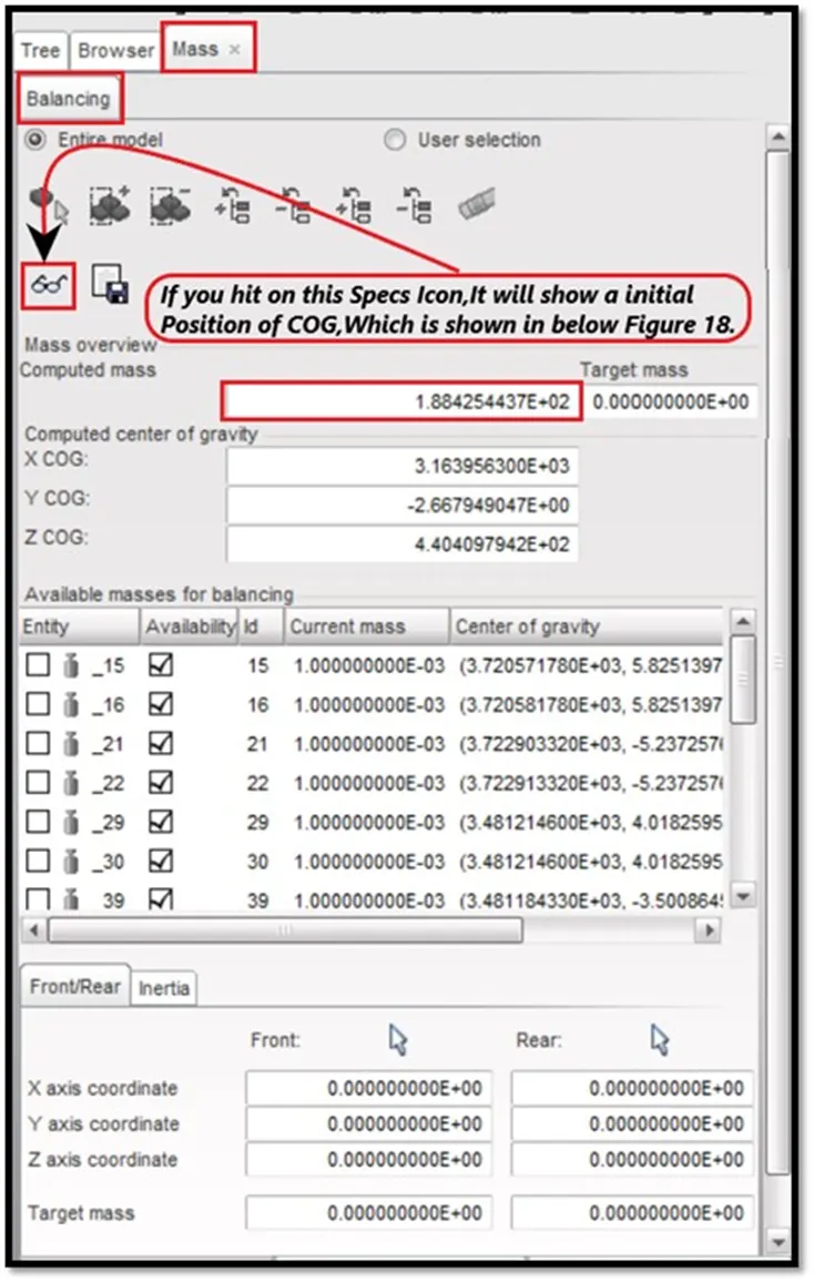
After hitting on the specs icon which is shown in above Figure 16.The initial position of COG will appear.

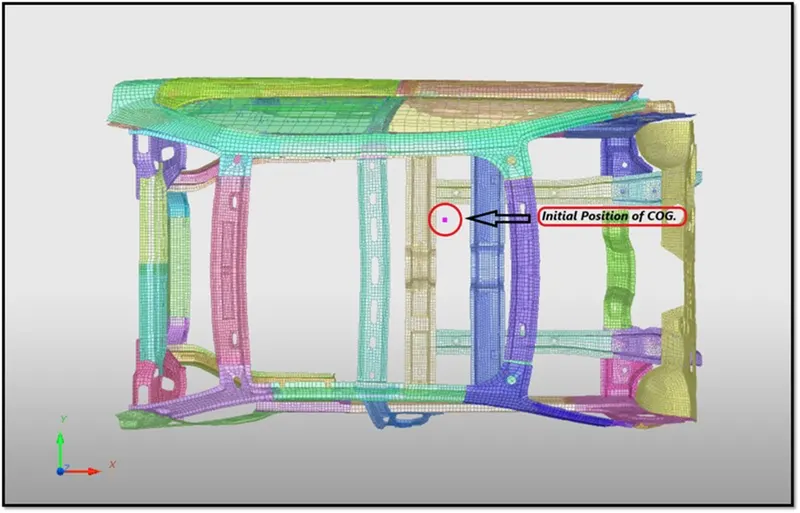
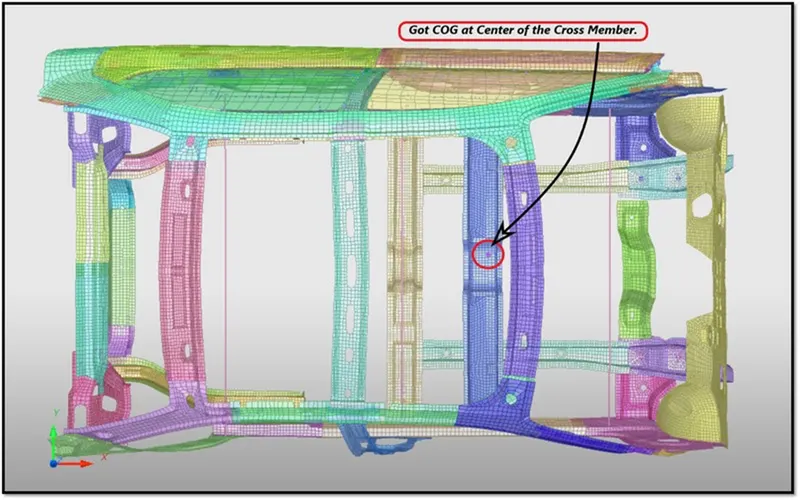
Now mass should be added to get COG in a proper position.It should be in centre of the cross member.

To bring COG to the centre of the cross member,We should add a mass.

To add mass Go to Load Case >> Added MassWhich is shown in below

Now right click on the added mass browser and select Type=0,Where the mass will be added to every single node,

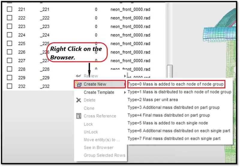
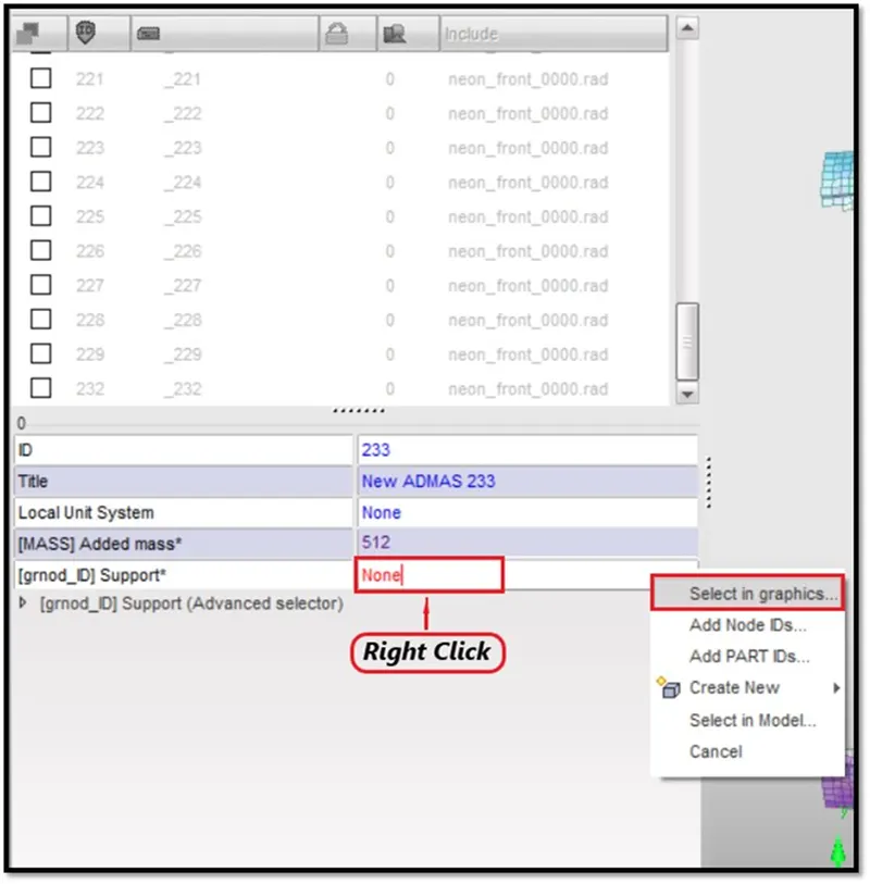
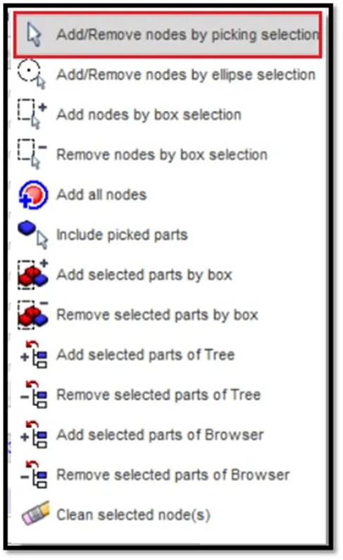
Here right click on the [grnod_ID] Support* to pick the nodes to add mass,

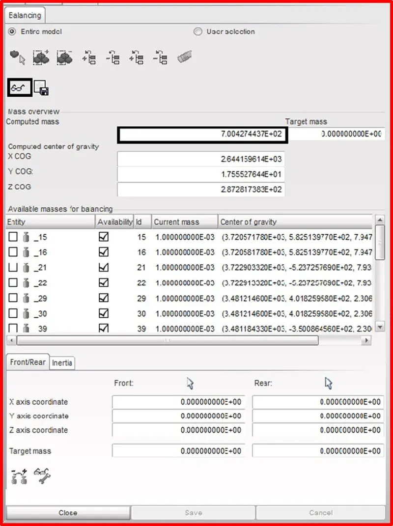
Now export this file and save it in a specified location and import this model into hypermesh and check the total mass.

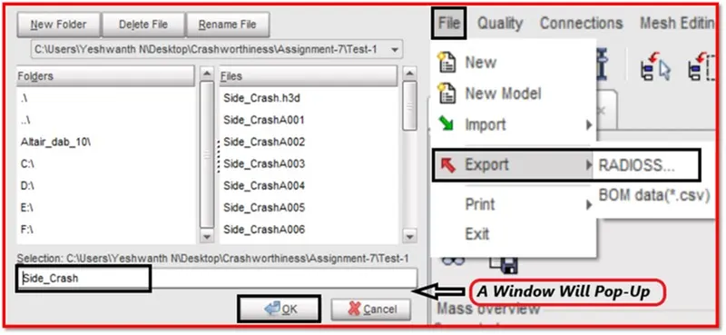
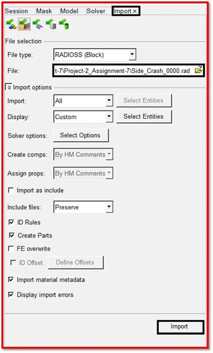
Now import the exported model from HyperCrash to the HyperMesh.

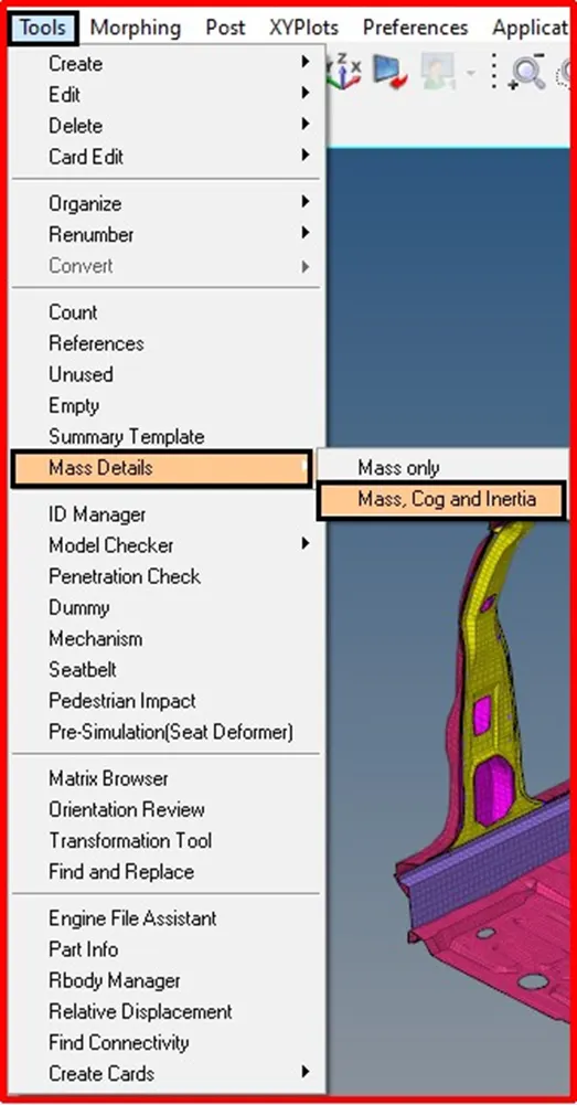
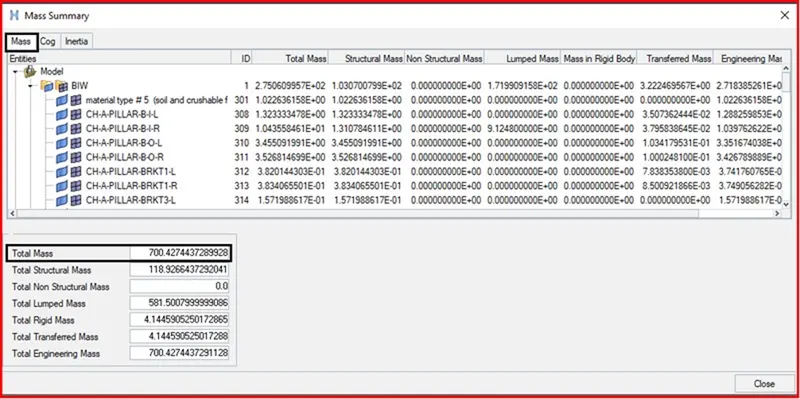
Next go and check in hypermesh,Whether the we have attained 700 kg mass.

To check,Go to Menu Bar >> Tools >> Mass Details >> Mass,COG,Inertia.

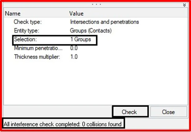
Next select the groups [Interfaces] to define.Which is shown in below.

Then click on the check to check penetrations in the model,If the penetration exsist,It throw a error in the status bar,If the penetration dosen't exsist,it will display No Collisions Found which is shown in below.

Phase 4-Create the Interfaces :

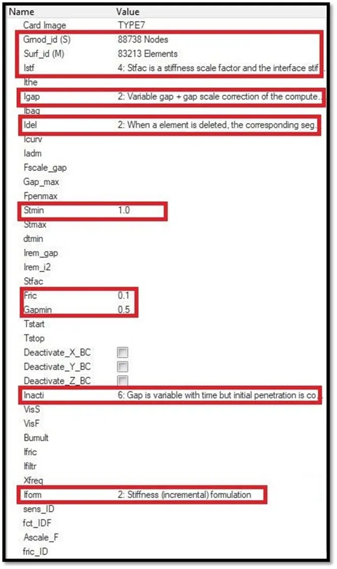
Here for this model,TYPE 7 Contact Interface is created with the recommended parameters.Which is shown in below.

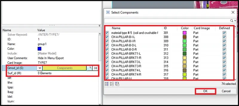
Select the slave and master nodes by switching to the coponents and select all the components for slave and master nodes which is shown.

Phase 5-Creation of Section at Cross Member :

Here we have to create a section,the section should be created at the cross member.

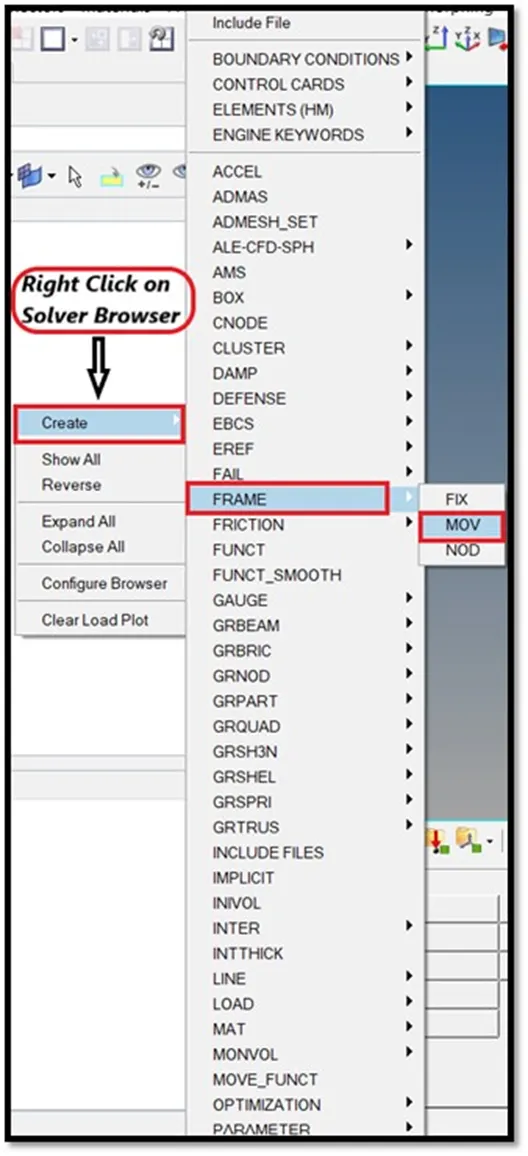
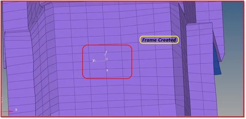
Next for creating section,We need frame,So we need to create frame first.To create frame Right click on the Solver Browser >> Create >> Frame >> Mov. which is shown in below

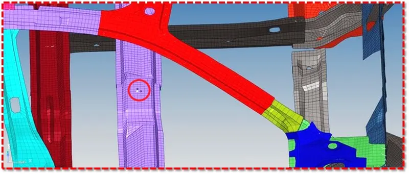
Next select the nodes to specify the location of the frame to be created on the model.

Switch to the create by node reference,Now select the Node at Origin >> Node at Z-axis >> Node at YZ Plane,

The Nodes selected to create a frame at a specified location is shown in below

Then create a section,To create a section,Right Click on the Solver Browser >> SECT >> SECT.

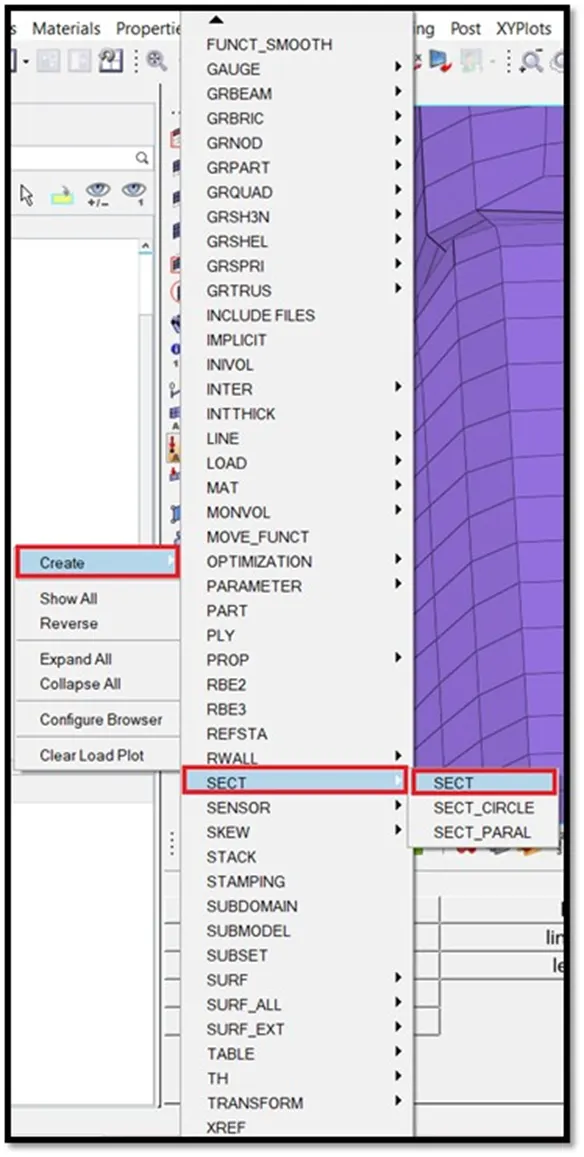
After selecting the SECT to create section,A parameter window will be opened left side.

There will be Nodes (N1,N2,N3),Select the nodes to create a section.Which is shown in below

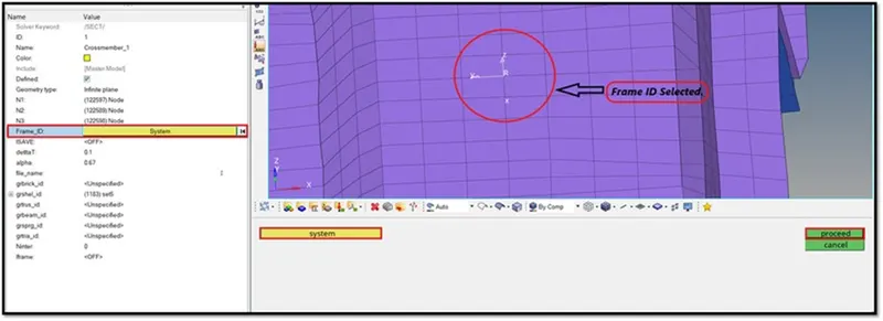
Next select the Frame ID,Which is shown in below.

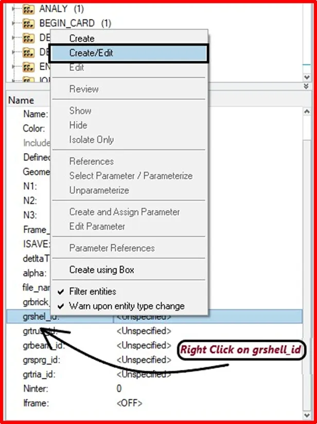
Next Right Click on the grshell_id to select the elements,where we created the section.Which is shown in below.

Enter the values for deltaT and alpha.

Coefficient of filtering (alpha=0.67).

Time step for saving the data (deltaT=0.001).

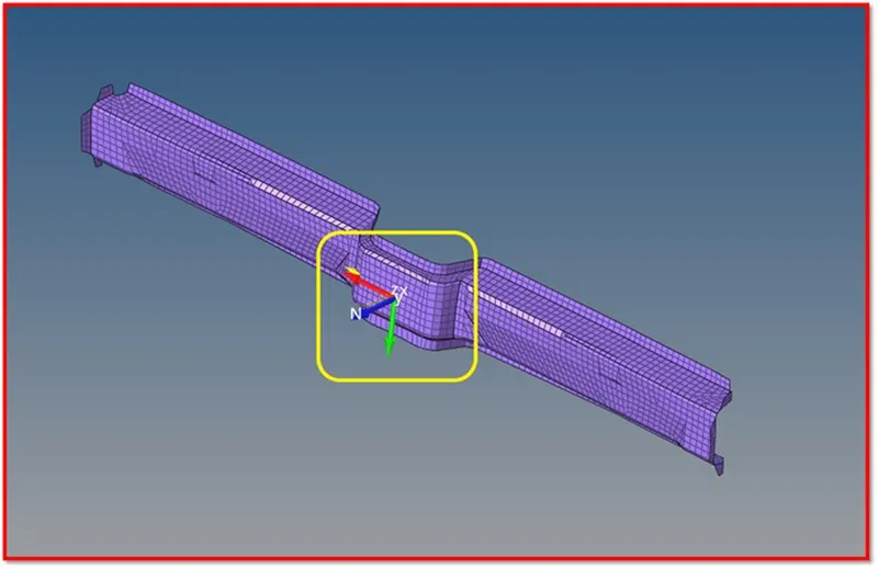
Now we have to check whether the section created for the rail component is fine or not fine.

If all the nodes get realized in the elements,then the section created for rail component is fine.Which is shown in below.

A one row of elements should be maintained.

To check Right click on the Section in the Model Browser >> Review.

Phase 6-Creation of Intrusion at B-Pillar,Hinge Pillar and Fuel Tank Region :

Here we have to create intrusions at B-Pillar,Hinge Pillar and Fuel Tank Region.

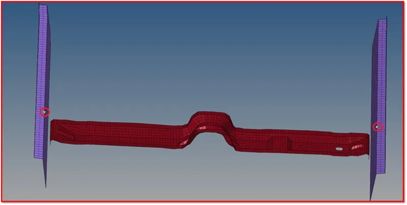
First we have to create spring 1D element,To create,First create a temp node on the B-Pillar base component.Which is shown in below

Next step is translate this node to other left B-Pillar,Cause to create spring,We need two nodes,So translate the node and create a temp node parallel to the,where the node created on the right side of B-pillar,Create a temp node with the reference of translated node.Which is shown in below

Phase 7-Create Initial Velocity :

Now we have to give the initial velocity to the car.

So to give the initial velocity we have to create INIVEL.

To Create,Go to Solver Browser >> Right Click >> Create >> Boundary Conditions >> INIVEL.

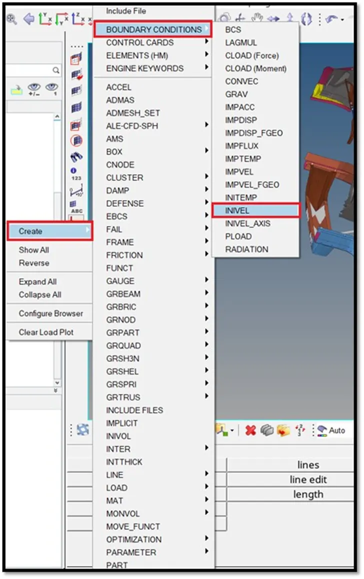
So,We want the car body to move in the x-direction so we have to give the velocity in the x-direction only.

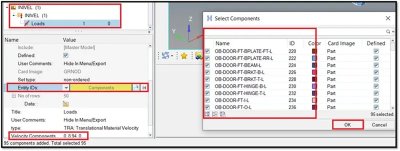
We need to give the velocity as 20 mph which we have to convert into the m/s. So after converting the velocity we got the velocity as 8.94 m/s.

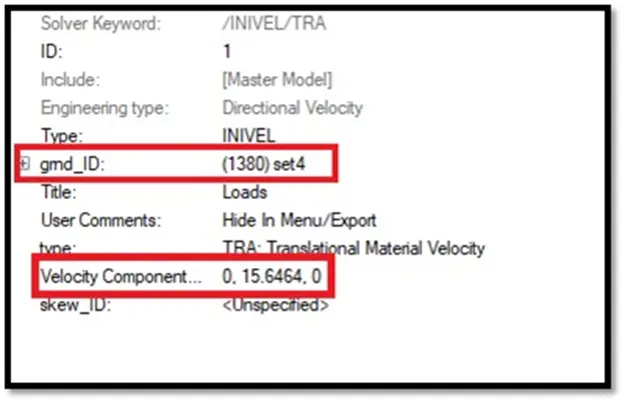
Right Click on the gmd_ID and select all the components,Cause whole car body want to move in x Direction.Which is shown in below

Phase 8-Create Peak Velocity of Inner Node of the Door :

Here we have to create a peak velocity,To create a peak velocity,First we have to create a node.

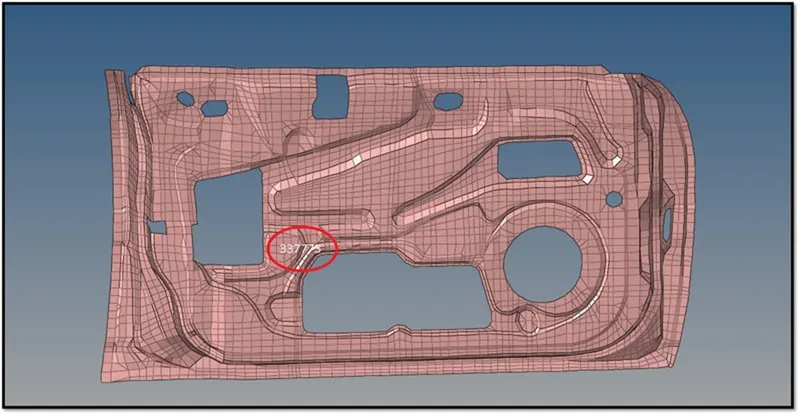
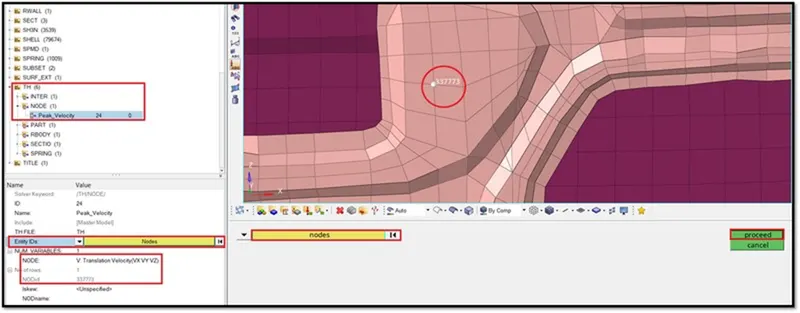
We have to give peak velocity at the given node [337773].

To find the node,Go to Display Panel.To find we have to display the numbers in the display panel.Which is shown in below.

Select the node by id and eneter the id number and click on which is shown in below

The node number is displayed,Which is shown in below

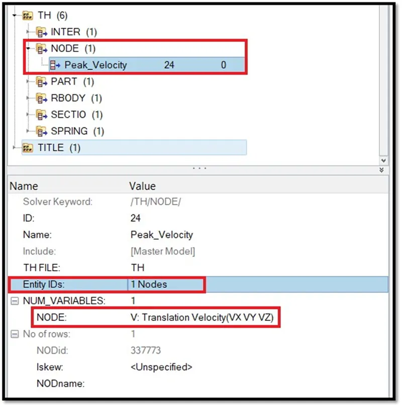
Next,Create a TH for that node. Because,to know the peak velocity at that point.

So,We have to request TH for that Node.

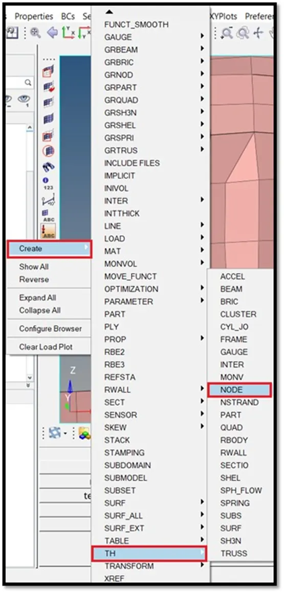
To create a TH for that node, Right Click on the Solver Browser >> Create >> TH >>NODE.

Phase 9-Create rigid wall with friction 0.1 :

Here we have to create cylindrical rigid wall,Cause this side pole crash,So.

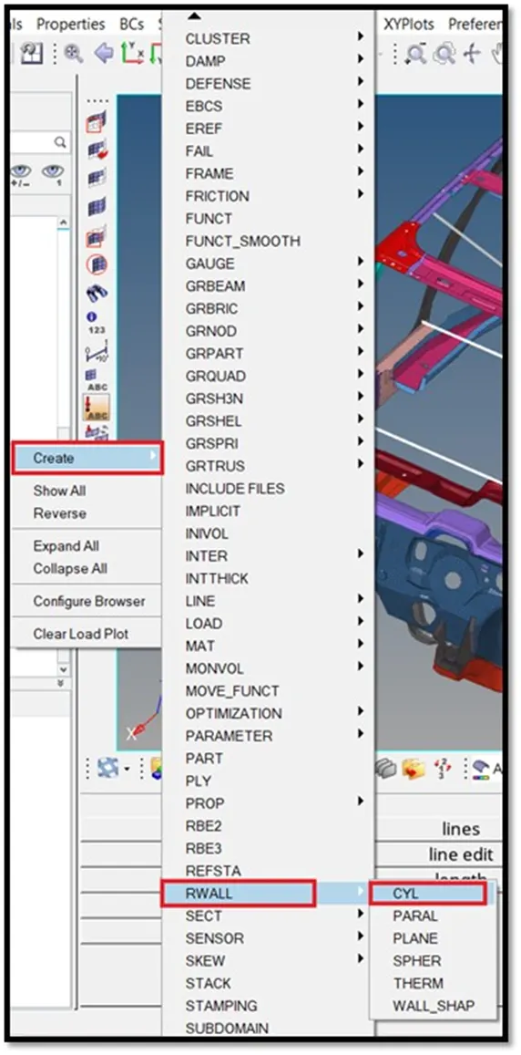
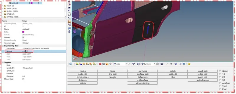
To create Rigid Wall,Right Click on Solver Browser >> Create >> RWALL >> CYL.

Next we have to create a temp node on the car door to make a cylindrical rigid wall.

After creating a temp node,Translate that node to the 300 mm.

After translating a node,In the RWALL parameter window,We have to select (XM,YM,ZM).It is selcted by,Clicking on the node which was translated which is shown in below Figure .

And the few parameters such as Friction, diameter of the cylindrical pole (Rigid), Searching tolerance(Dsearch) should be given which is shown in below Figure.

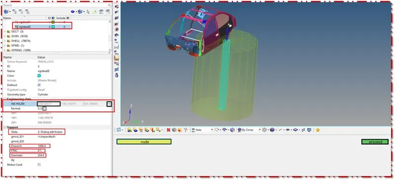
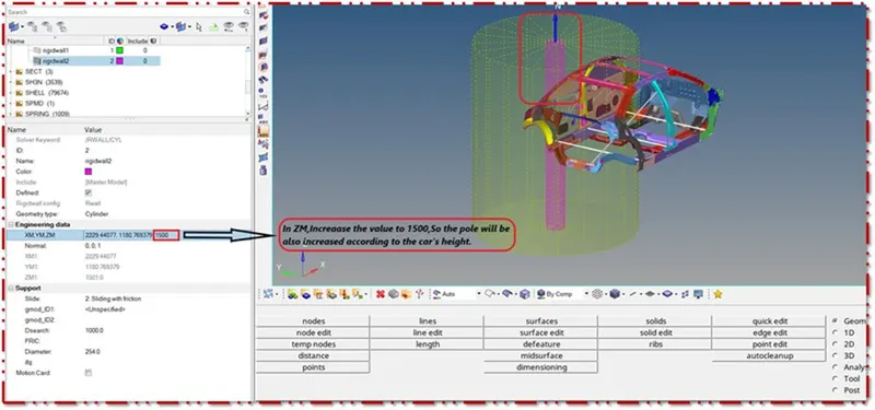
Here increase the value of ZM to 1500 to increase the height of the rigid pole to the car's height which is shown

Phase 10-Run the Simulation :

Now run the simulation,To run simulation,Go to Analysis Panel as shown in below.

Go to Analysis Panel >> Radioss >> Select the Input File >> Save it in Different Folder and Rename it as Test-1 >> Run.

Check the Include Connectors,If there are any connectors in the model,The connectors will also be taken into account.

Type -NT 4 in options tab,This will make the simulation faster.

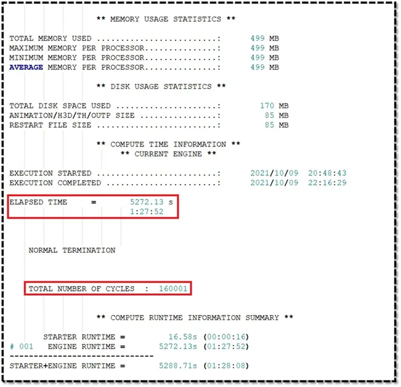
After completing the simulation,the radioss will pop up a solver window stating Radioss Job Completed which indicates the simulation has been completed.

Here the number of animation steps obtained are shown in below

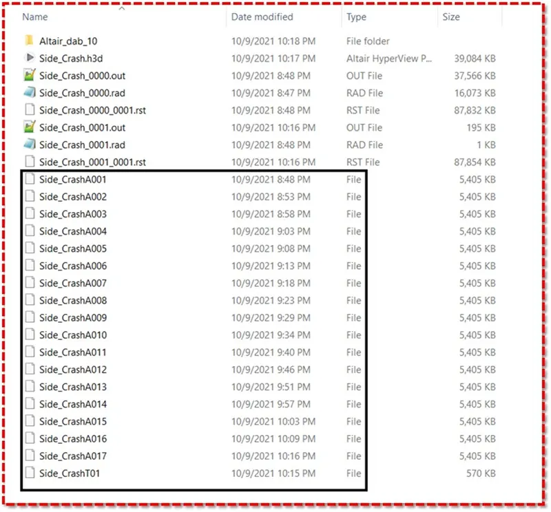
Now go and open the 00001.out file with notepad.

The obtained values for Energy Error,Mass Error,Internal Energy Error,Kinetic Energy Error and Contact Energy Error has been shown

1) Review the Simulation using HyperView :

Hyperview allows for loading and viewing result files obtained from several sources.

Based on the solver type of the files and the results you would like to visualize and analyze,there are differnt ways to load the input deck and their corresponding results into hyperview.

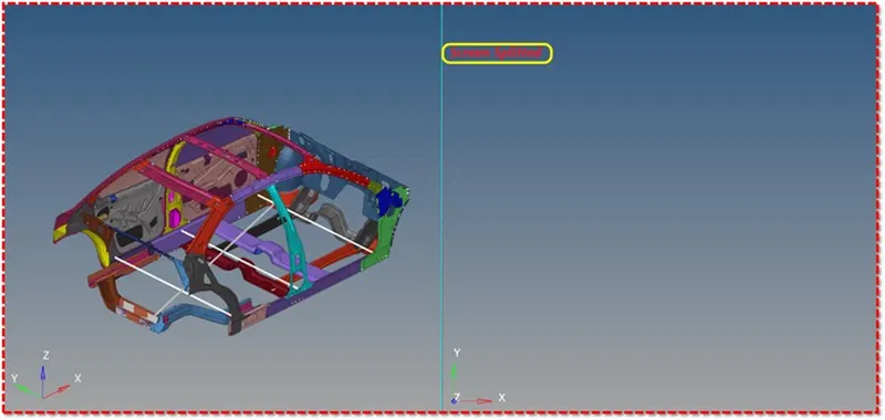
First to begin the postprocessing in the Hypermesh,Split the Screen as shown in below Figure 100.

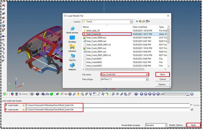
Import the animation file .h3d into the hyperview.

To access the load model panel

Select Load Model Button from the HyperView Panel and open .h3d file as shown in below

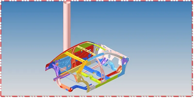
After loading the model into hyperview,It will be represented as shown in below

After importing the .h3d file into the GUI,Enable the contour.

The contour tool create contour plots of a model graphically visualize the analysis results.

To enable contour,Go to Results ToolBar >> Contour

Now switch to the Von Misses Stress in result type and select the component,select the averaging method as simple and then click apply as shown in below.

After applying ,Run the Simulation,The Simulation animation in terms of Elements,Von Misses Stress and Displacement is shown in below

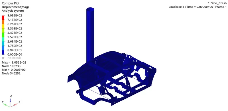
Here the contour plot displays the displacement of each node of the BIW model of a car in a GUI.

Displacements are computed with respect to the global co-ordinate system.

As the model crashes into the rigid pole,the deformation occurs to each nodes and the nodes gets displaced from their initial position.

During the simulation,maximum displacement occured at node 190233 which is shown in above

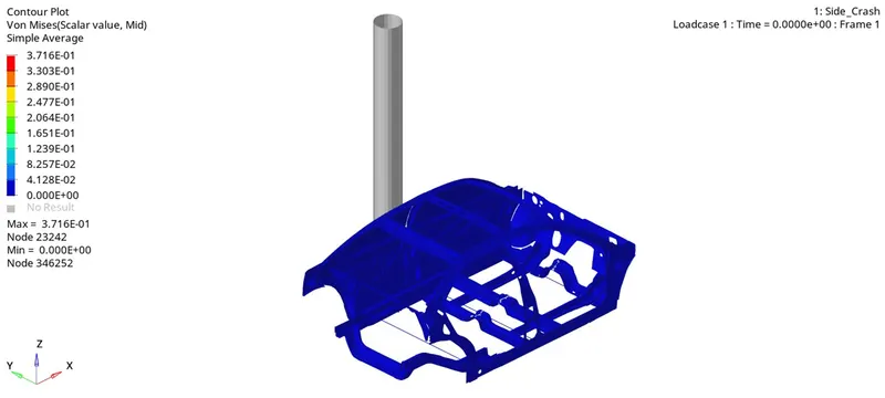
Here the contour plot gives the stress induced at each node in the BIW model of the car.

As the model crashes,internal stress is developed in the model due to the material behaviour.

During this simulation,The maximum stress developed at each node is 23242 which is shown in above

After defining the nodes at the end of the spring after the collision,

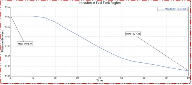
Intusion at Fuel Tank Region:

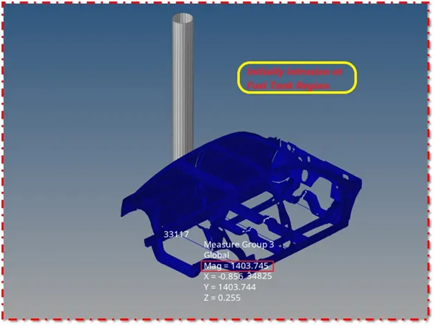
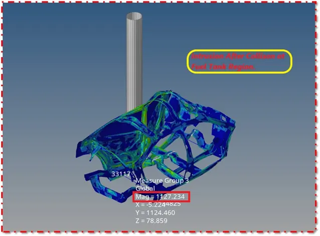
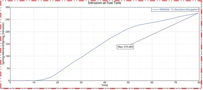
Intrusion at Fuel Tank Region is 1403.745-1127.234 = 276.511 mm.

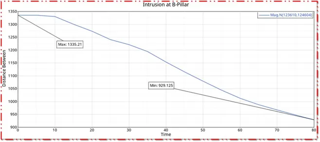
Intusion at B-Pillar Region:

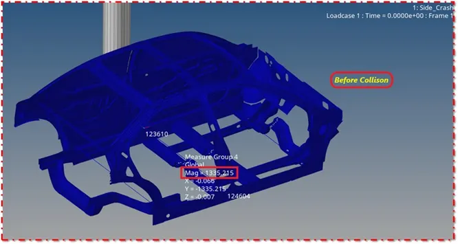
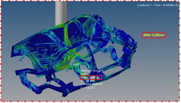
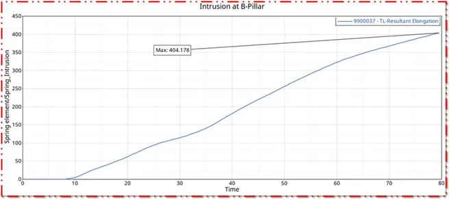
Intrusion at B-Pillar Region is 1335.215-929.125 = 406.09 mm.

Intusion at Hinge-Pillar Region:

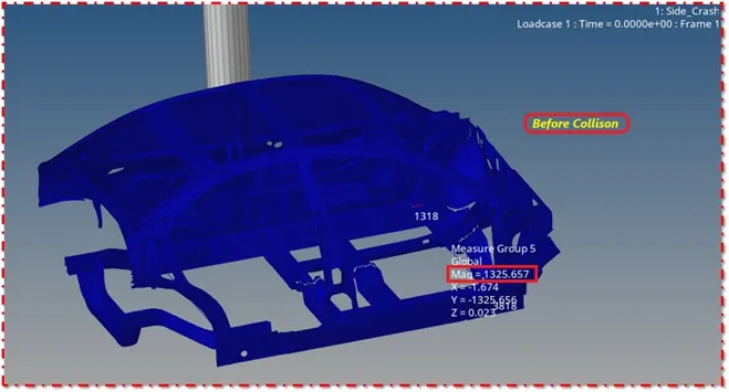
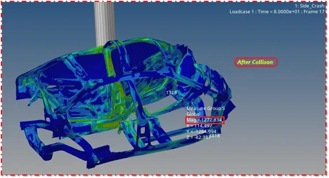
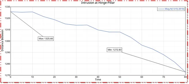
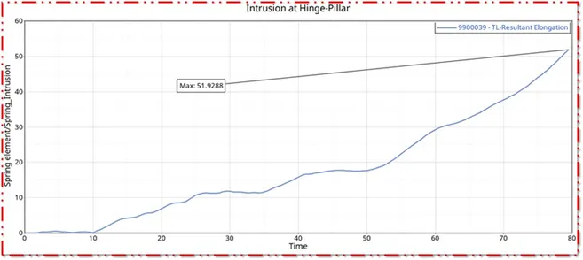
Intrusion at B-Pillar Region is 1325.657-1272.834 = 52.83 mm.

Plot the graphs using -Hypergraph 2D :

Now plot the graphs using Hypergraph 2D,We are plotting the graphs to see what is happening in the rail component.

Hypergraph 2D is a powerful data analysis and plotting tool with interfaces to many popular file formats.

It is sophisicated math engine capable of processing even the most complex mathematical expressions.

Hypergraph 2D combines these features with high quality presentation output and customization capabilities to create a complete data analysis system for any organization.

Intrusion Graph for Fuel Tank Region :

Here the graph is obtained for the Fuel Tank region which is shown in below.

In the beginning,the length of the spring was 1403.74 mm and after when the car crash the pole,the length of the spring is 1127.23 mm.So the total deflection of the spring is 276.511 mm.

Intrusion Graph for B-Pillar Region :

Here the graph is obtained for the B-Pillar region which is shown in below.

In the beginning,the length of the spring was 1335.21 mm and after when the car crash the pole,the length of the spring is 929.125 mm.So the total deflection of this spring is 406.09 mm.

Intrusion Graph for Hinge-Pillar Region :

Here the graph is obtained for the Hinge-Pillar region which is shown in below.

In the beginning,the length of the spring was 1325.66 mm and after when the car crash the pole,the length of the spring is 1272.83 mm.So the total deflection of this spring is 52.83 mm.

Peak Velocity :

The graph obtained for the peak velocity is shown in below

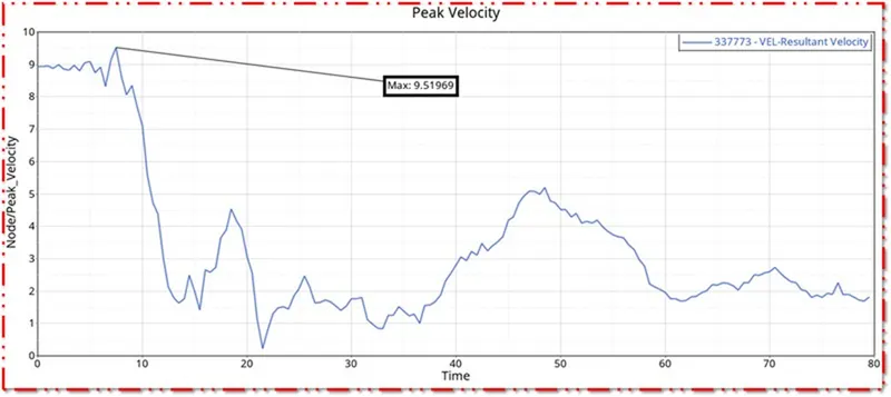
When the car hits the pole,the door will be deformed,So due to the deformation,the inner portion of the door will hit the passengers inside the car and it may cause severe injuries to the passengers.

So it is important to calculate the peak velocity at the door region.

The peak velocity of the node on the door is 9.51m/s.The graph is in Zig-Zag form,Due to the noise and vibration,When the the car hits the pole.

Here the the velocity is starting from peak due to the initial velocity is given and it goes on decreasing,cause the car goes and hits the pole,due to deformation,itse decreasing.

We gave the initial velocity as 8.94 m/s,But in the graph,the initial velocity is 9.51 m/s,It's increased little bit,Because due to inertia.

Interface [TYPE 7] :

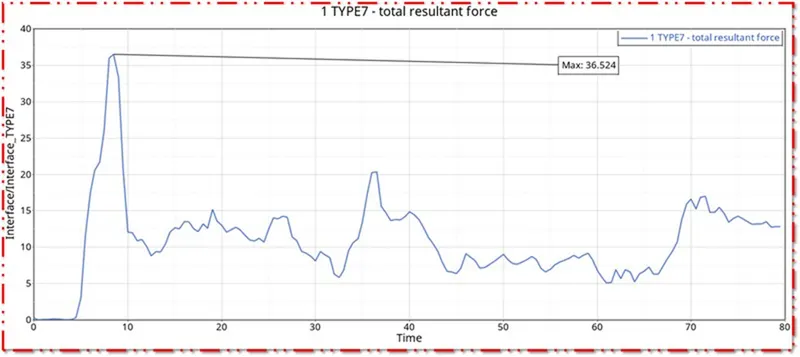
The graph obtained for the Type 7 - Total Resultant Force Interface is shown in below.

Here the interfaces curve starts from origin and reaches peak due to collision.

And it increases & decreases before it reaches to peak value,Cause there will be a contact forces acting with in the car before collision.

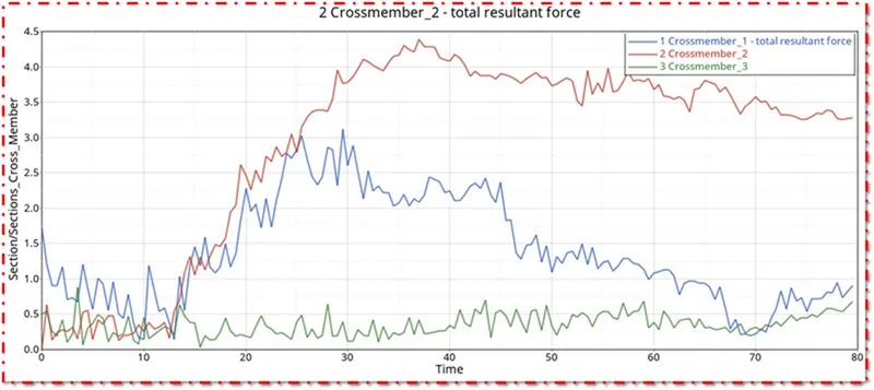
Variation in Sectional Forces

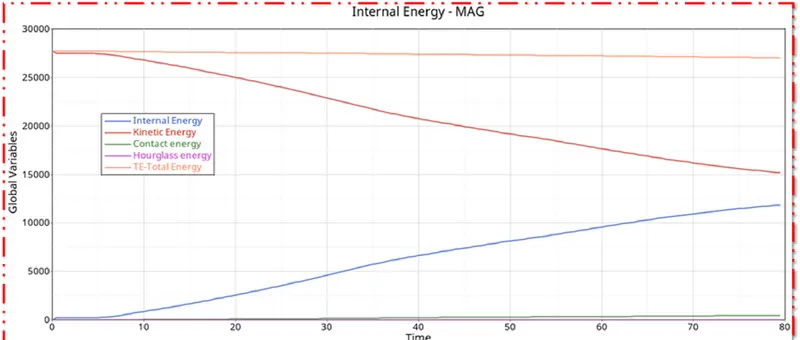
All Energies :

All the energies have been plotted which is shown in below

Kinetic energy:

The graph obtained for kinetic energy is shown in below

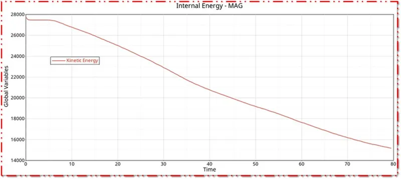
Kinetic Energy is at peak in the starting,Why because,we have huge mass.

Kinetic energy is lower and decreases,why because,there is a velocity applied to the car component,so its getting deformed and the kinetic energy decreases.

The kinetic energy will decrease due to the decrease in velocity after the collison,When the car hits the rigid pole. So,the kinetic energy decreases with respect to time.

Internal Energy :

The graph obtained for internal energy is shown in below

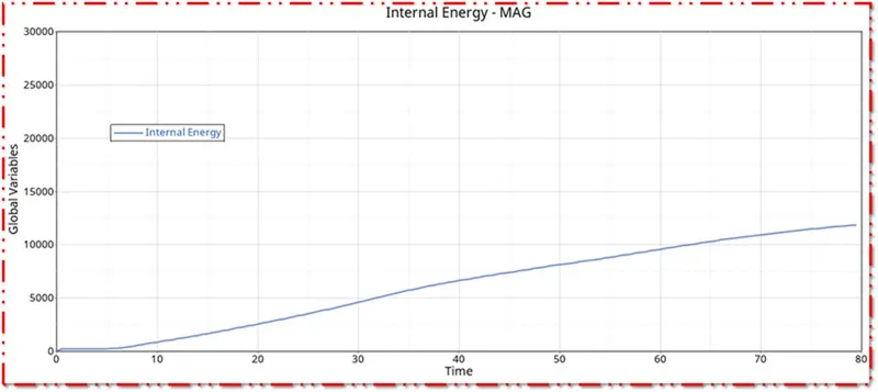
The formula for Internal Energy is I.E = Q W.

Here the heat is neglected,Cause there is no heat transfer,We will be having only workdone.
W=FxD
F=ma

Here the internal energy is in Zero,Because there is no deformation initially,So the internal energy is in Zero and starts from Zero and goes on increasing.

The internal energy increases because the deformation is happening,there is a displacement,So the internal energy increases,when the displacement or deformation occurs.

Contact Energy :

The graph obtained for Contact Energy is shown in below

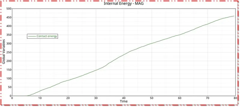
Here the contact energy starts from origin,Cause the Car is in intial condition.

Intially there is no contact between the Car and Rigid Pole.

There is also no deformation intially,But when the car goes and hits on the rigid pole,The contact energy starts increasing.

When the deformation or displacement happens to the car,the contact energy increases,cause the car component comes within the contact to the rigid pole.So the contact energy goes on increasing.

Total Energy :

The graph obtained for Total Energy is shown in below

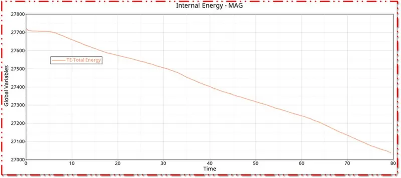
Total Energy is sum of Kinetic Energy+Contact Energy+Hourglass Energy + Internal Energy.

Here total energy starts from higher value,In starting itself its increasing,Why because the total energy is sum of Kinetic Energy+Contact Energy+Hourglass Energy + Internal Energy.

All energies are in initial condition except kinetic energy,So kinetic energy is only there

Total Energy=Kinetic Energy+0+0+0.

Kinetic enrgy is directly proprtional to the total energy.

So the total energy is increasing in the beginning.

Due to -1.8% of energy error,the total energy is decreasing.

Hourglass Energy :

The graph obtained for Hourglass Energy is shown in below

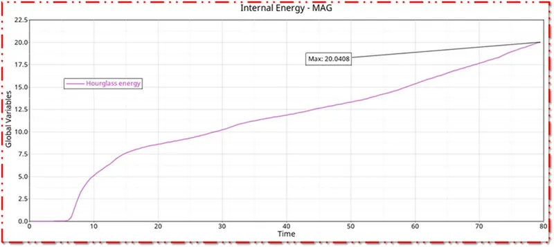
Here the hourglass energy is less than 5% of internal energy,So it is fine.

RESULTS:

• Hence the COG from the initial position has been changed to the required position by mass balancing.
• Hence the penetrations and intersections has been verified successfully.
• Hence the interfaces created newly.
• Hence the peak velocity has been given to the inner node.
• Hence the initial velocity was assigned.
• Hence the rigid pole was created successfully.
• Hence the TH for all inputs were created inorder to obtain outputs.
• Hence the simulation was runned successfully without any errors.
• At last all the graphs were plotted with the obtained results.