Frontal crash analysis on Dodge neon car BIW using FMVSS 208 standards
Objective
Perform the frontal car crash simulation on the neon car model.
In this project, we are going to make sure that there is no penetration and intersection in the model. Create the rigid wall with the friction of 0.1. We have to add the mass in the car to make the total mass of the car to be 700 kg. We have to create sections and check the sectional forces there. We have to create an accelerometer. We have to check the intrusion in the given part of the body.
Introduction
BIW
Body-in-white (BiW) is the name given to a car body’s sheet when all its components—barring moving parts (e.g., hoods, fenders, etc.), trims (e.g., glass, seats, etc.), or chassis subassemblies—have been welded together. Usually, BiW constitutes about 27% of a car’s curb weight and remains the key determinant of how the car will perform.
Frontal Crash
The objective of a crash test is to measure how well a passenger vehicle would protect its occupants in the event of a serious real-world frontal crash. Federal Motor Vehicle Safety Standard (FMVSS) No. 208 is the measure that gives us the valuers that how much it can be deformed so the passenger should not get injured that much. If it is within the limit then we can say that the car has passed the test otherwise it is failing.
The ideal frontal crash test procedure will be able to evaluate occupant protection while ensuring that the vehicle will not jeopardize its crash “friendliness” with its collision partners. Finally, the test conditions (e.g., impact speed, impact angle, and test device) must be representative of the frontal crash environment to which passenger vehicles are exposed on the highway.
There are some tests we can perform in the frontal crash analysis. In one analysis, the vehicle is projected towards a solid obstacle at a predesigned velocity. The obstacle can either be a concrete wall or a barrier., NHTSA is amending its safety standard on occupant crash protection to establish 56 km/h (35 mph) maximum speed for frontal barrier crash tests.
Another version of the frontal impact test involves a crash between two vehicles. In this type of testing, we crash two cars and check what happened to the vehicle and the passenger. Physical testing is very expensive so what car manufacturers do is perform more tests that involve a solid obstacle. That's when proper design and Computed simulations come into the picture. Real tests are just for approval of simulation results. Hence save a lot of money.
There are some offset tests also done in the frontal crash analysis of the car. In this type of test, only a part of the car impacts the obstacle, whether it’s a wall, barrier, or another car. This test is extremely important because even though the impact area isn’t as large, the impact forces are almost as high as with the full-frontal crash.
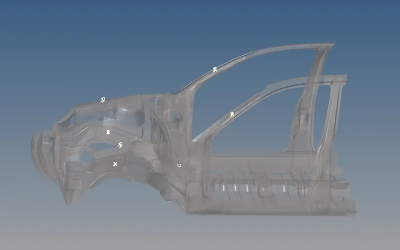
So we are going to do the frontal crash in which we are going to do the crash of the car on the wall. So our analysis is the Full Frontal Fixed Deformable-face Barrier (FFFDB) test. In this test, we are going to give the velocity to the car to be 54 km/h (35 mph). We are going to create the intrusion and we are going to check the deformation in the intrusion so that we can see that it is failing for the crash or it passed the test.
Procedure
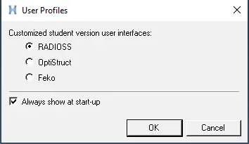
1. We are going to choose the profile to be Radioss.
2. Now we are going to import the model.
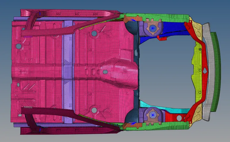
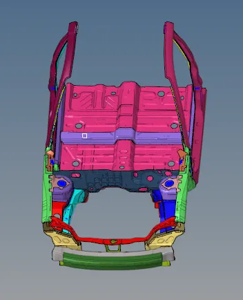
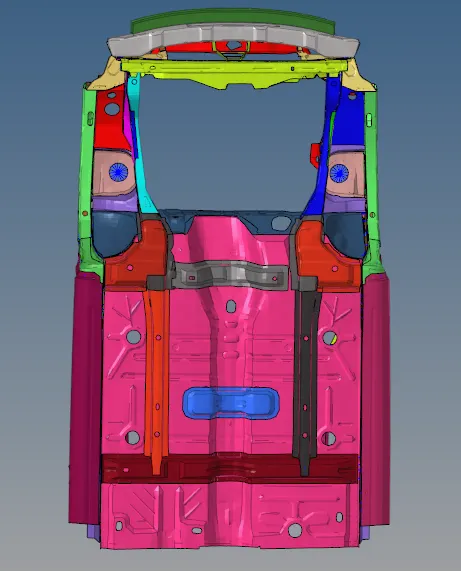
3. Now we are going to check the unit of the model. For that, we will go to the BEGIN_CARD.
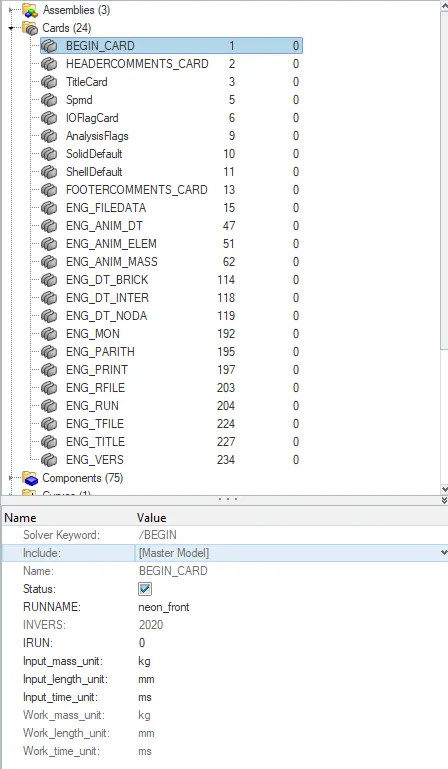
So the unit of the system is in kg, mm, ms.
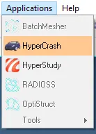
4. Now we will go to the HyperCrash. To go there Application--> HyperCrash
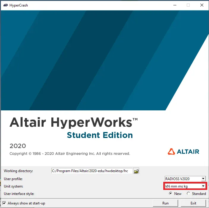
We have to make sure that the unit system of the HyperCrash is in the [ kN, kg, mm, ms].
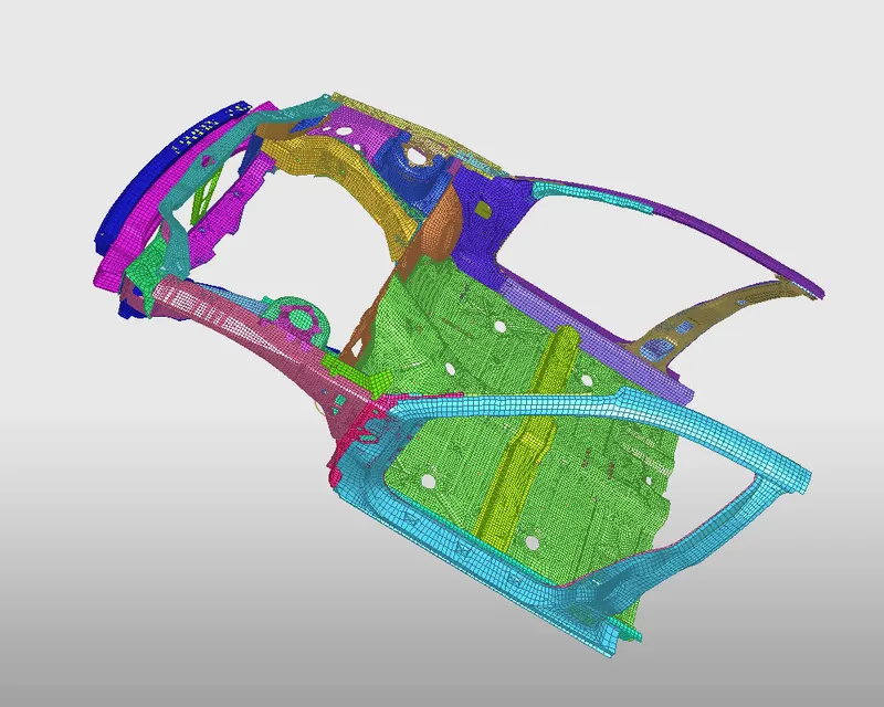
Now in the HperCrash to import the model we are just going to drag and drop the 0000.rad file. That will do the work.
5. Now we are going to check if there are any penetration and intersection in the model. For that we will go to the Quality--> Check All Solver Contact interfaces
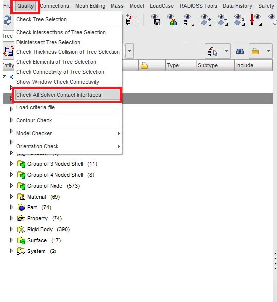
After click on the option HyperCrash check for the penetration and intersection and show us the result.
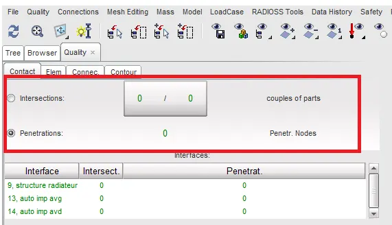
So there is no penetration and intersection present in the model.
6. Now we are going to check the mass of the model. In order to that, we will go to the mass--> Balancing
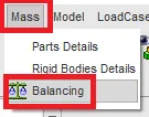
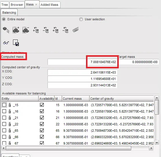
So after selecting the balancing option we can see the mass of the model.
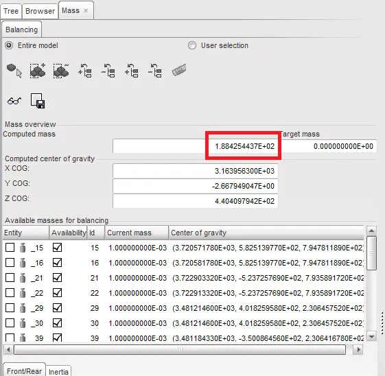
It is showing that the total mass of the body is 188.2 kg which is 700-188.2 = 511.8 kg less than our target mass.
To check the COG of the body we have to click on the specs icon.
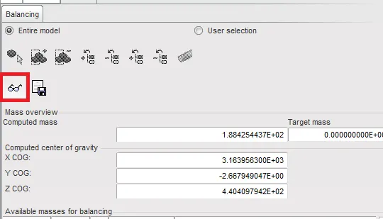
So the COG of the body is at the point which is showing in the below picture.
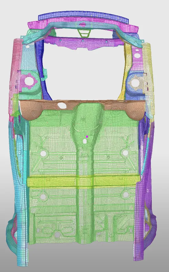
7. We need to increase the mass of the body to be 511.8 kg and get the CG of the body to be in the required range we have to add the mass very carefully.
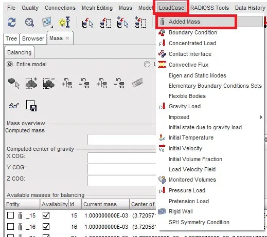
To add the mass we will go to the LoadCase--> Added Mass.
8. Now to add the mass we are going to click on the create on the new object in that we are going to add the mass and the nodes where we are going to add the mass.
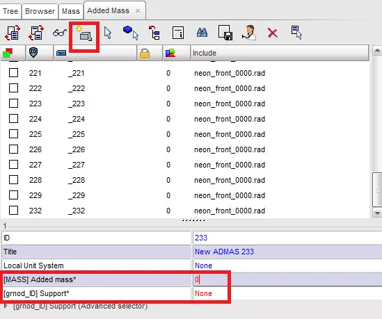
We have to be very careful in adding the mass so that the CG of the model should be on the required area and we got the target mass of 700 kg of the model.
After adding the mass:-
And CG of the model:-
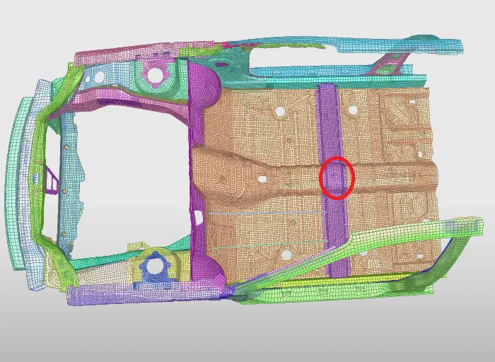
Now we have achieved the target mass of the car and we have got the COG in the required area.
9. Now we are going to export the model so that we can do the rest of the work in the HyperMesh. To export the model we will go to the File--> Export--> RADIOSS
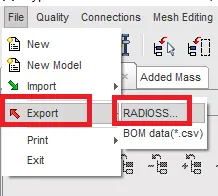
Now we are going to save the file in the "0000.rad" format. And we are going to open that file into the Hypermesh.
10. Now in Hypermesh we are going to give the model a type 7 self contact. To create the contact we will go to the solver and we are going to create it.
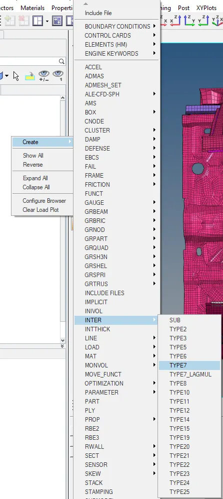
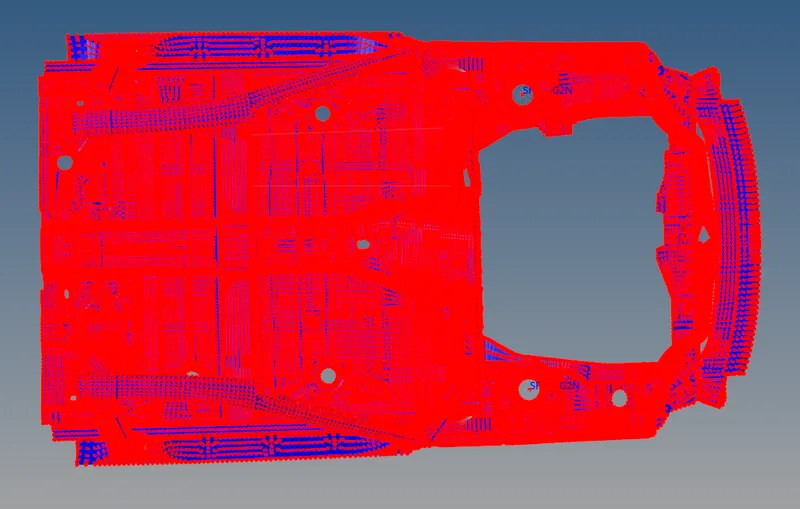
In the contact, we are going to give the master and slave nodes. It is a self contact so we are going to take the master and slave nodes to be all nodes of the car model.
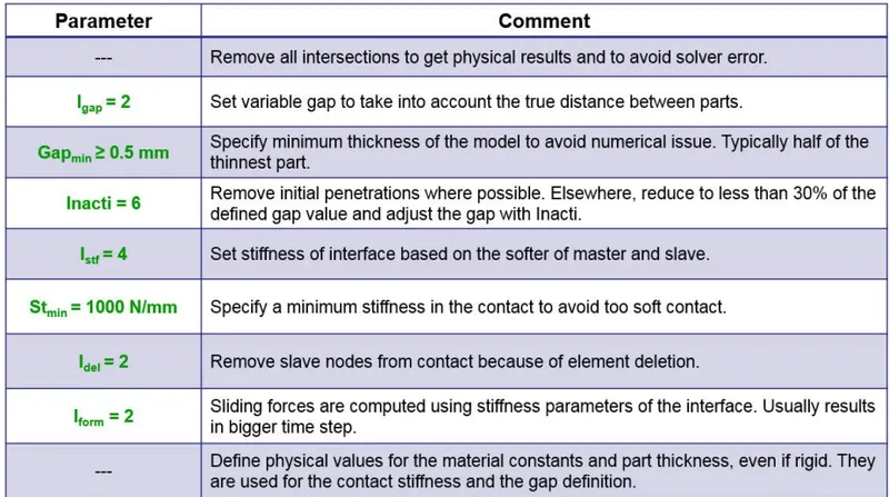
We are going to give the recommended value to the interface.
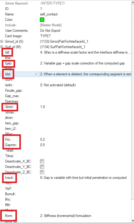
We are going to take the friction to be 0.2 because it is given in the problem so instead of the recommended value we are going to give friction to be 0.2.
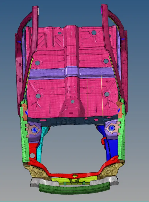
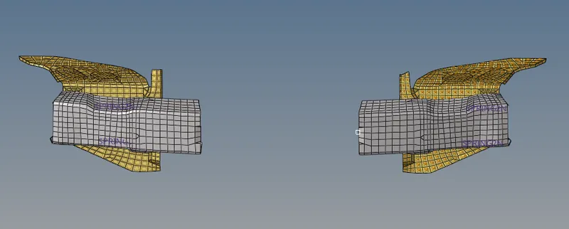
Similarly, we have to give the type 7 contact between the Bumper and the component near to that with the same properties.
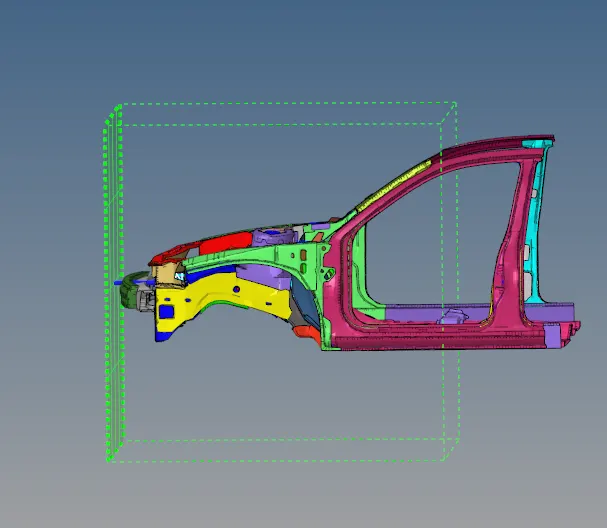
11. Now we are going to create a rigid wall.
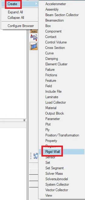
In the rigid wall creation, we have to give the coordinate of a base point of the surface where we want to create the rigid wall and we have to give the normal vector coordinate.
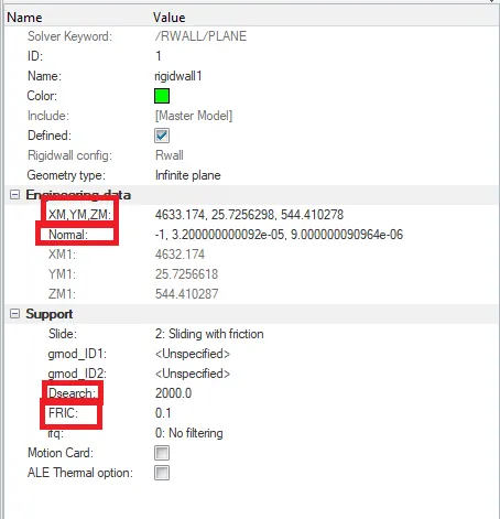
We have to give the friction of the wall to be 0.1. We are going to give Dsearch value to be 2000. Dsearch value is the value that gives us the search tolerance of the master and slave nodes near the wall.
12. Now we are going to give the initial velocity to the car. So to give the initial velocity we will go the create--> Boundary Condition --> Inivel
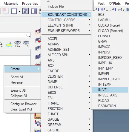
In the initial velocity first, we are going to select the node where we want to give the initial velocity. We want the whole body to move so we are going to select all the nodes of the car model.
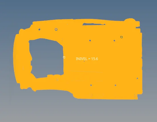
We want the body to move in the x-direction so we are going to give the velocity in the x-direction only. We need to give the velocity to be 35 mph which we have to convert into the mm/ms. So after converting the velocity we got is 15.6464 mm/ms.
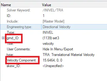
13. Now we want to calculate the sectional force in the rails at node 174247 and opposite to the node (left and right rails). cross-sectional forces on the shotgun (left and right shotgun). We need to calculate the cross-sectional forces on the A-pillar of the car.
So we have to create the sections on these points. In order to create sections, we are going to need frames. So first we are going to create the moving frames in these points. In order to create the frame we will go the create--> Frame--> Mov
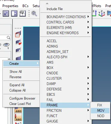
And we are going to create the frame on the required points. In the creation of the frames, we are gonna required the origin node then we are going to define the x-axis after that we are going to define the XY plane.

So the frames:-
14. Now we are going to create the sections so that we can check the forces on these points. So to create the section we will go to the Create--> Sect--> Sect
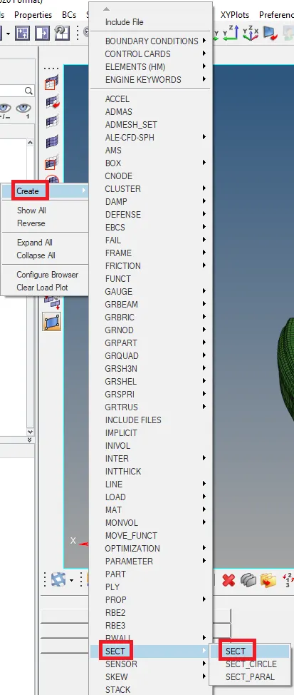
So while creating the section we have to select the frame and we have to select the elements which is near to the frame.
We are going to give the alpha value to be 0.67 and the delta T value to be 0.001.
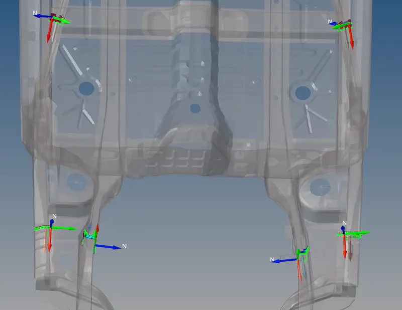
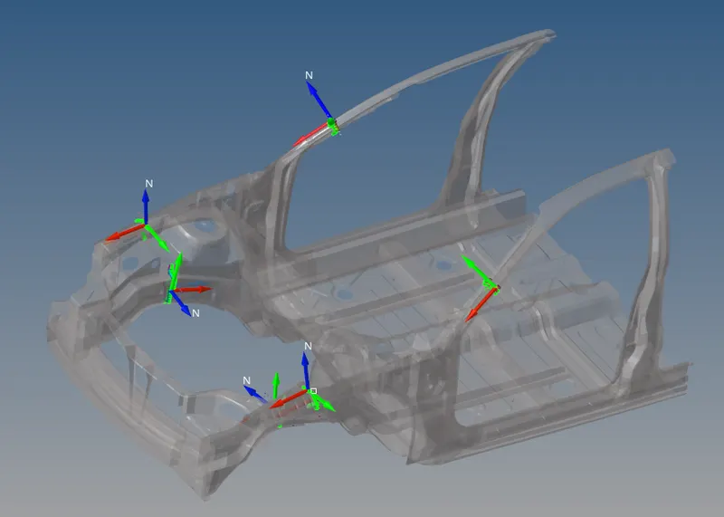
So we have created the required section in the model.
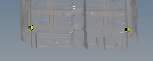
15. Now we are going to create the accelerometer on the B pillar (left and right B pillar rocker). So in order to create the accelerometer, we will go to create--> Accelerometer
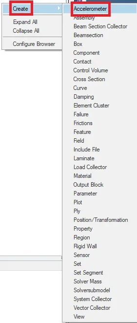
In the accelerometer, we just need to give the node location where we want to create the accelerometer.
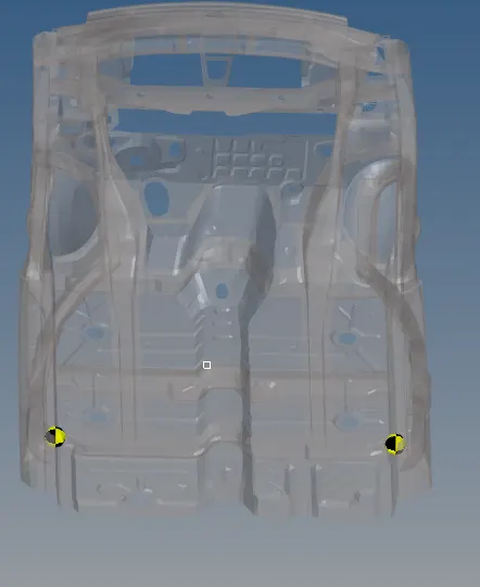
16. Now we need to create the Intrusion on node points 66695 and 66244. So instead of that, we are going to create the spring on those points.
So to create the spring we will go the 1D--> Spring

In that, we are going to create the spring between two nodes.

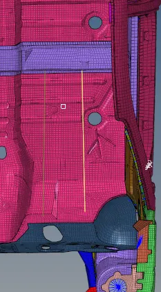
We have to give some property to these springs. In the property of the springs, we are going to give the mass of 0.001 kg and stiffness of 0.001 N/mm.
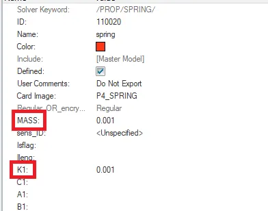
Now we have to assign the property to both springs.
17. Now we are going to check the connectivity of the model. We don't want any component of the model to be free. Because if there is any free component that remains on the model after the crash they will go fly away. That is bad for our simulation. We want the components to be connected for better results.
So to give the connection we will go to the 1D--> rigids


After we select two or more nodes, those two components will be connected by an RBE2 (Rigid Body Element) that will hold those components in place. An RBE2 element has infinite stiffness, it will not deform under excessive loads.
18. Now we are going to create TH file to get the required output. We need TH file for the springs, accelerometer, sectional forces and, contact forces.
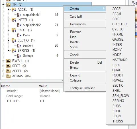
So we have created the TH file for all the required outputs.
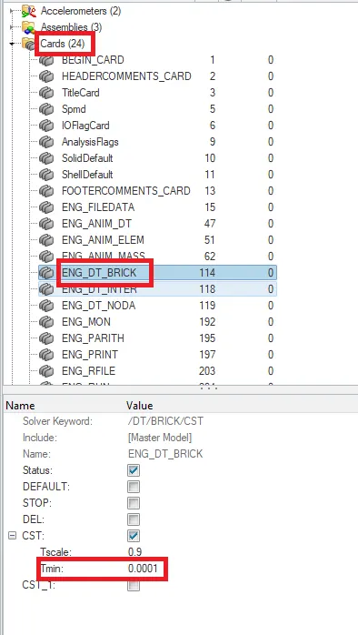
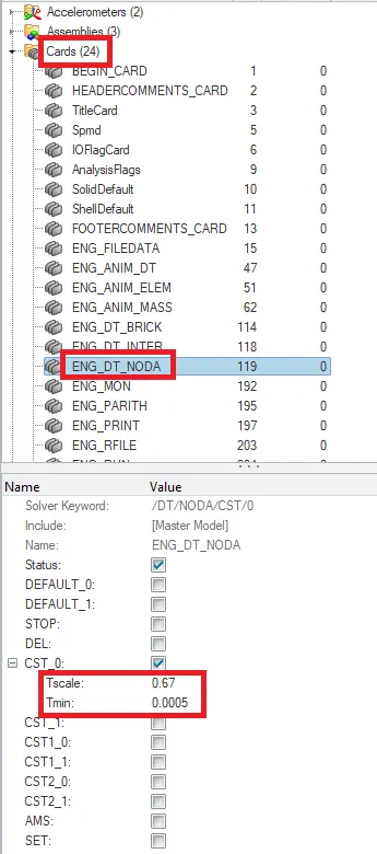
19. We need to give the time step value in brick to be 0.0001 ms.
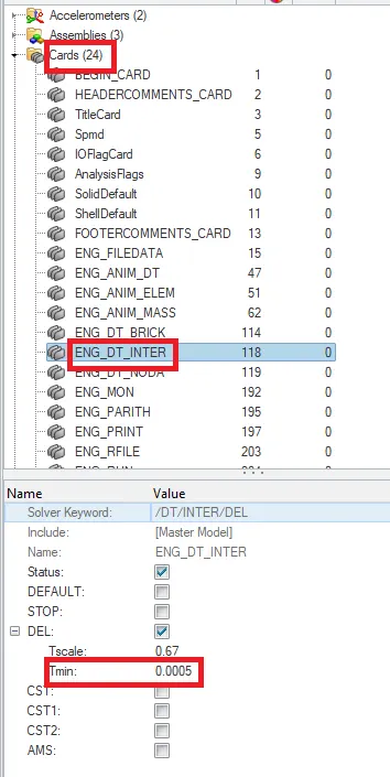
In inter to be 0.0005 ms.
And in the Noda to be 0.0005 ms.
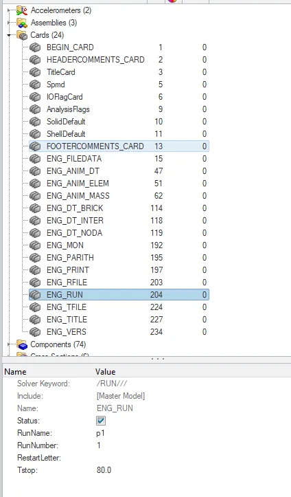
We want the simulation to be run for the 80 ms. So we are going to give the Tstop time to be 80.
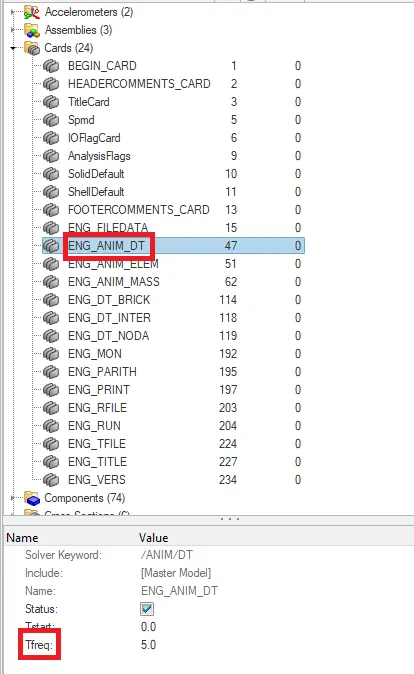
We are going to give the Tfreq to be 5.
20. Now we are going to run the simulation. To run the simulation we will go to the Analysis-->Radioss


Now we are going to analyze the simulation and we are going to plot the required graph.
21. To check the simulation we have done is correct or not we are going to check the energy error and mass error. If it is in the accepted range then we can say that our simulation is correct.

The energy error is between -15% to 5% and the mass error is 0. That is very less so we can see that the simulation we have done is right.
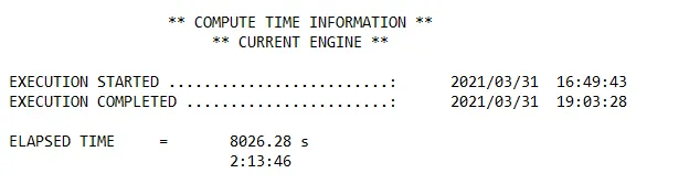
The total running time of the simulation was 8026.28 seconds.
22. Now we have to analyze the simulation frame by frame and check the behavior of the element after the impact.
Output
Simulation Gif
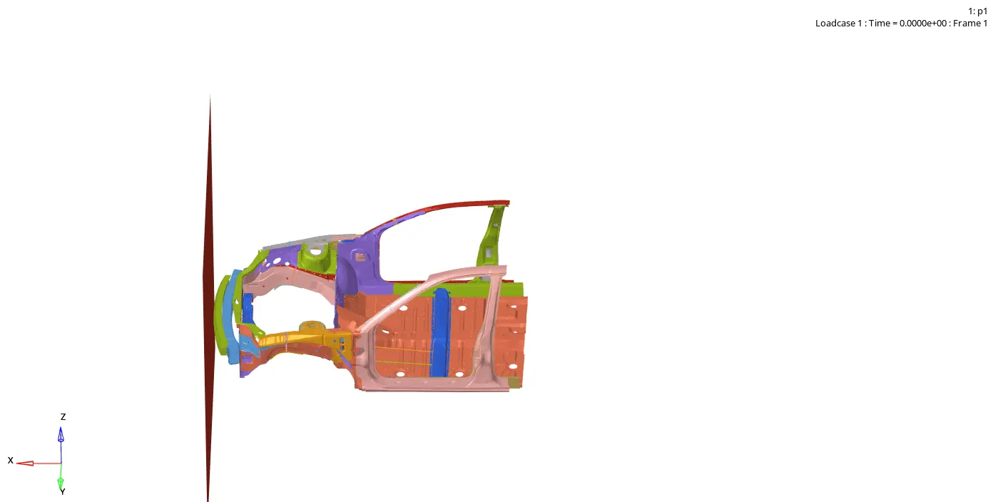
In this simulation, we can see that in the frontal crash how the elements are getting deformed. In the simulation, we can see that the elements in the front get deformed maximum and the elements which are in the rear of the model are going up.
Displacement Gif
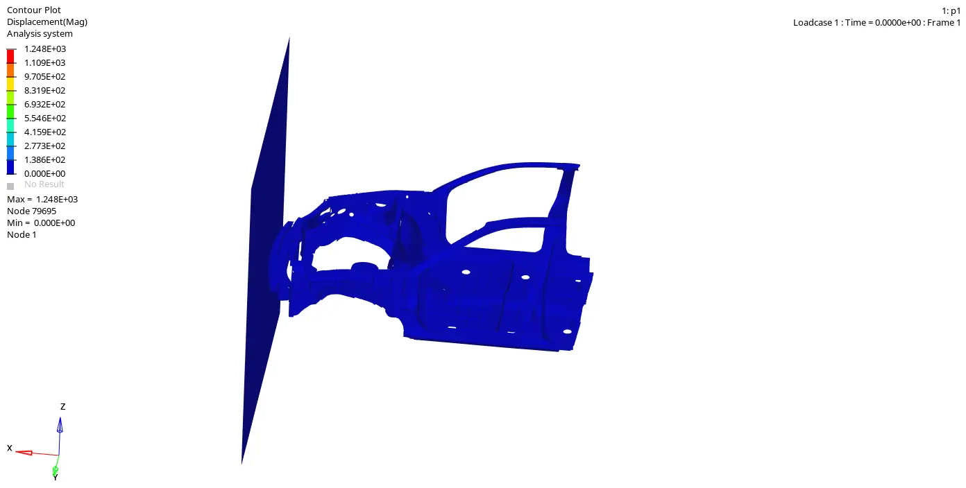
In this Gif, we can see that how many elements how much getting displaced. We can see that the elements which are in the front get displaced very less and the elements which are in the rear end of the model and gone up because of the crash are displaced more than any of the other elements.
Von Mises Gif
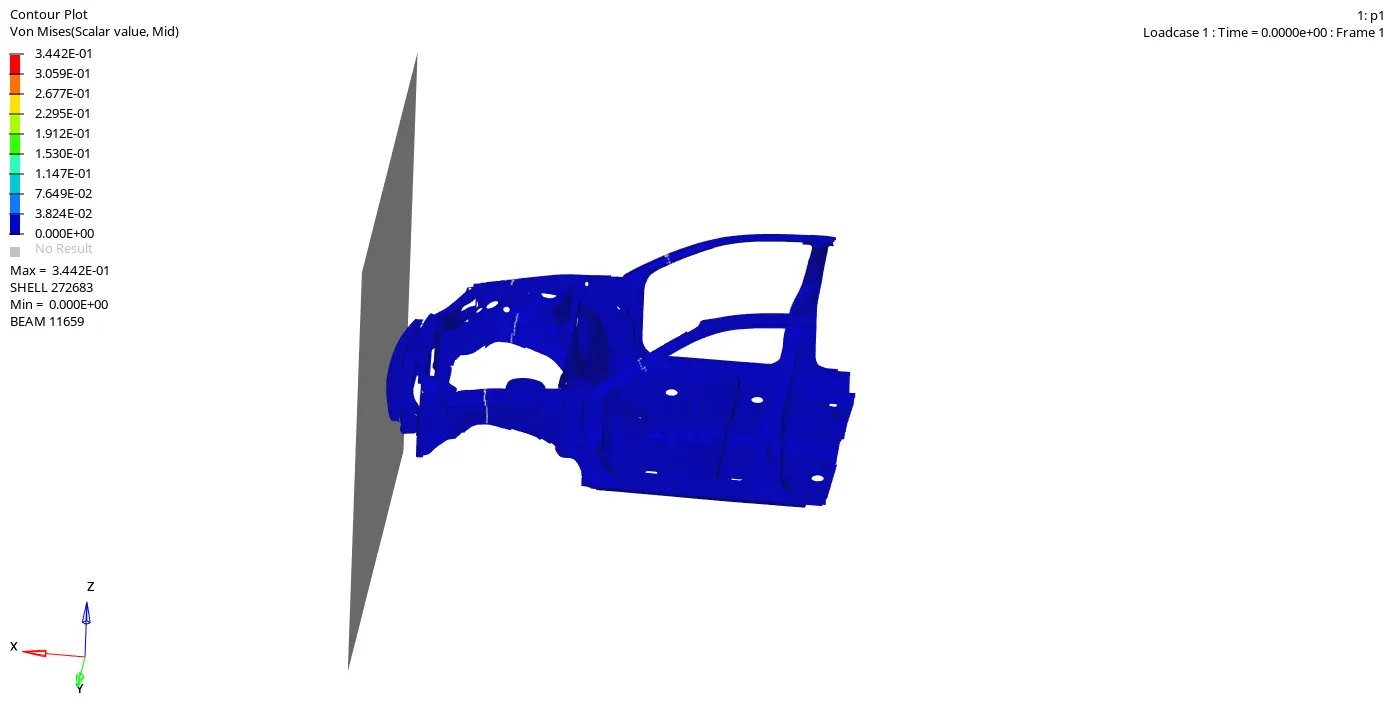
Von Mises stress is a value used to determine if a given material will yield or fracture. It is mostly used for ductile materials, such as metals. The von Mises yield criterion states that if the von Mises stress of a material under load is equal or greater than the yield limit of the same material under simple tension then the material will yield.
Energies
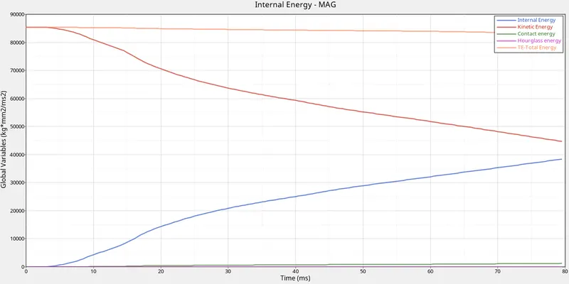
From the above graph, we can see that with the time, when the model gets impact on the wall the velocity of the model decreases, and because of that the kinetic energy also decreases. The internal energy of the model gets increases with time.
The total energy is the sum of the kinetic energy and the internal energy. So because of some contact energy, the total energy is decreasing at the end of the simulation.
Contact Energy is the energy due to contact between two elements. So when the deformation occurs elements start to get in contact with each other so due to contact between elements we get the contact energy. We are getting very low contact energy in the simulation.
We have taken the shell element to be QEPH so we get hourglass energy to be zero.
Acceleration Curves
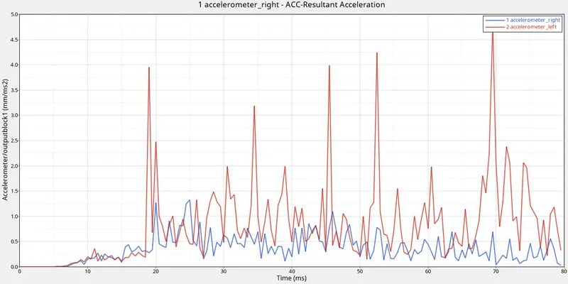
From the graph, we can see that the acceleration in the left B pillar was more as compared to the right B pillar of the model. We can see that in the simulation also. The maximum acceleration recorded in the left accelerometer was 4.797 mm/`ms^2` and in the right accelerometer it was 1.325 mm/`ms^2`. So we can say that the elements which were on the left pillar side get deformed fast as compared to the elements which were on the right pillar side.
Sectional Forces
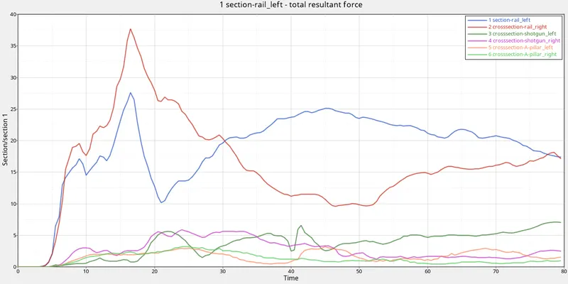
To check the forces on some particular area we have created sections. We have created two sections in rails (left and right), two in the shotgun (left and right), and two sections in the A-pillar (left and right). So in the above graph, we can see that how much of the forces are getting in those sections.
So in the graph, we can see that in the right rail we are getting more forces as compared to the left rail. The maximum force on the right rail we get 37.69 N and in the left rail, we get 27.58 N.
When we talk about the shotgun, So in the starting of the simulation we were getting almost the same forces in both shotguns (left and right) but after 40 ms the forces in the left shotgun increase, and the forces in the right shotgun they get decreases. So at the end of the simulation, the forces we are getting in both shotgun was very high as compared to the forces at the beginning of the simulation.
When we check the forces on the A-pillar of the model. So we are getting the forces to be the same at the beginning of the simulation in both pillars. After 40 ms the forces in both pillars we are getting are different. But the maximum value of the force in both pillars we are getting is almost the same. The forces on the left pillar we are getting are high most of the time of the simulation. At the end of the simulation, the force decreases.
So if we compare all the sectional forces, we can see that the forces on the rails we are getting were very high. After the rails, those forces were getting distributing to the many parts of the body. That is why the forces we are getting on the shotguns and A-pillars were very low as compared to the rails.
Axial Forces
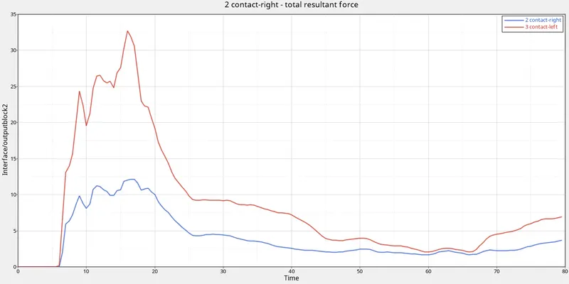
We have created type 7 contact between rails and bumper on both sides. So we get the axial force on the left side higher as compare to the right side. The maximum force on the left side was 32.694 N and on the right side, it was 12.155 N. The axial forces on the left side were always more as compared to the right side. It was maximum when they crash. But after 20 ms it decreases and remains very low.
Intrusions
To check that how much of the deflection is happening in a particular node, we create the intrusion there. There are two methods to create the intrusion. The first is by creating skew at a point and the second one is by creating a spring at that node.
When we create moving skew it moves with the node when there is deflection. So when the skew moves, the origin of the skew does not change. The origin of the skew is fixed. So we can check the coordinate of the skew and we can know how much of the deflection is happened at that point.
When we create the spring at a particular node. In that case, we can check how much of the length changes of the spring. So we get to know that how much of the intrusion is occurring at that point.
We are going to create two springs at the pedal area of the model to check the intrusion.
Left Spring
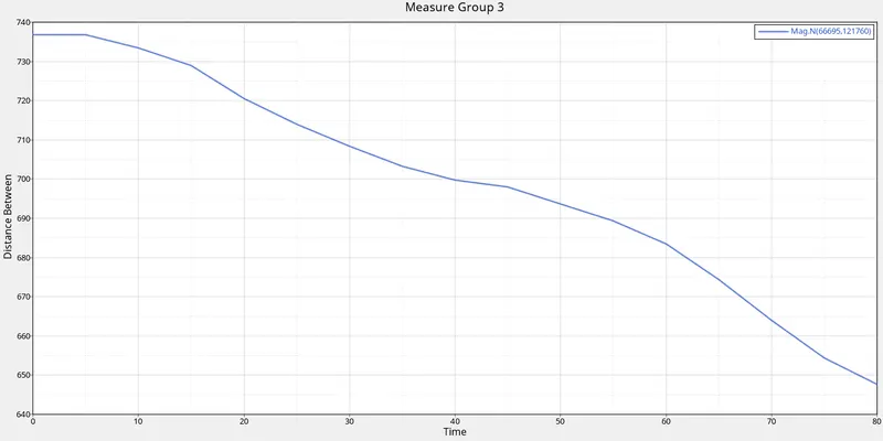
In the above graph, we can see that in the beginning, the length of the spring was 736.734 mm and after the crashing the length of the spring get 647.594 mm. So the total deflection of the spring is 89.14 mm.
Right Spring
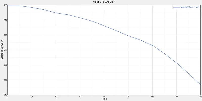
In the above graph, we can see that in the beginning, the length of the spring was 759.190 mm and after the crashing the length of the spring get 653.794 mm. So the total deflection of the spring is 105.396 mm.
According to the FMVSS 208 for a full frontal crash, max allowed intrusions are 15cm. We are getting the intrusion to be 89 mm and 105 mm which is less than 150 mm so the car has passed the frontal crash.
Learning Outcome
Learn about the frontal crash test and different types of frontal crash tests.
Learn about the FMVSS 208.
Learn how to add mass in the model and learn about the CG of the model.
Learn about the sectional forces, axial forces.
Learn about the accelerometer.
Learn about the intrusions.
Learn about internal energy, kinetic energy, hourglass energy.