Assignment 6-Frontal Crash Simulation Challenge
Aim: To perform the crash analysis according to the given conditions and obtain the desired output requests.
Procedure:
PRE-PROCESSOR (Radioss) :
- Import the model and check the unit system in the starter file.

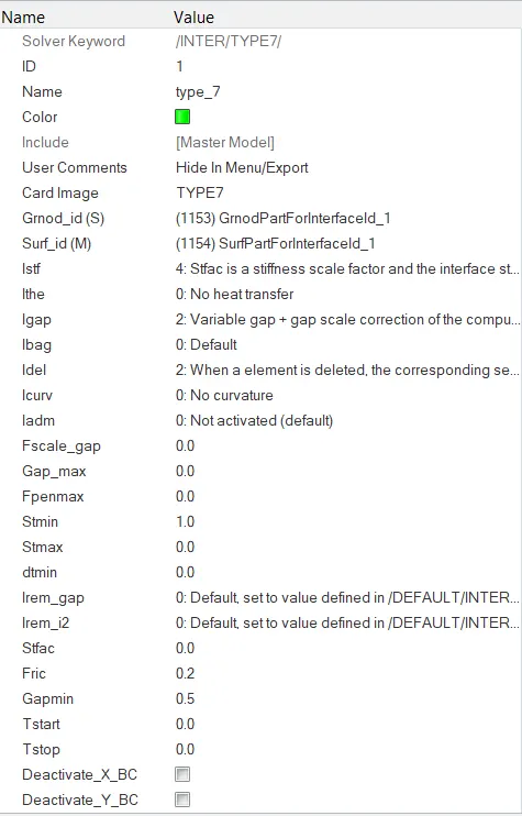
- Create a type-7 interface for the whole vehicle body by selecting all nodes and elems for slave master respectively.
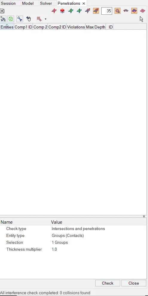
- Check for penetrations using the penetration checker in Radioss Tools-->Penetration check-->select group-->check
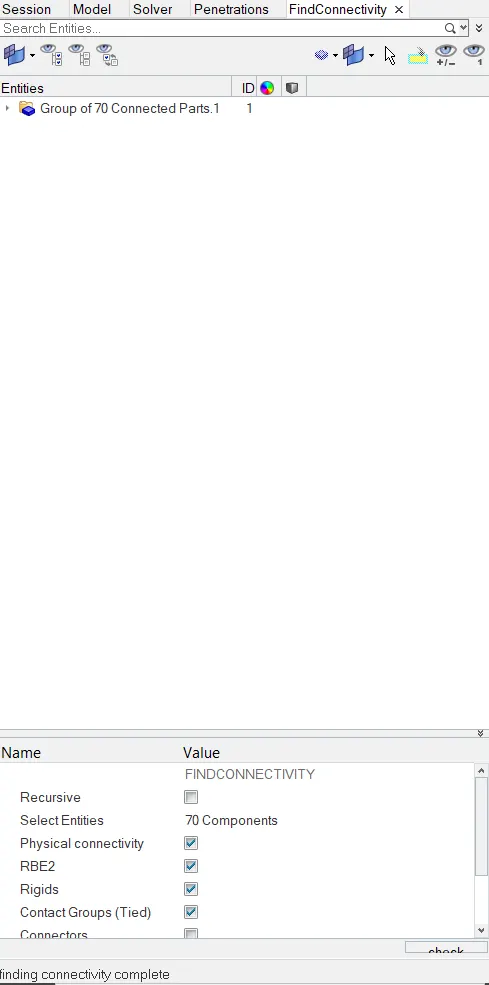
- Go to tools-->Find Connectivity-->select components and ensure that there are no free parts. If there are any delete them(translational joints, spherical joints)
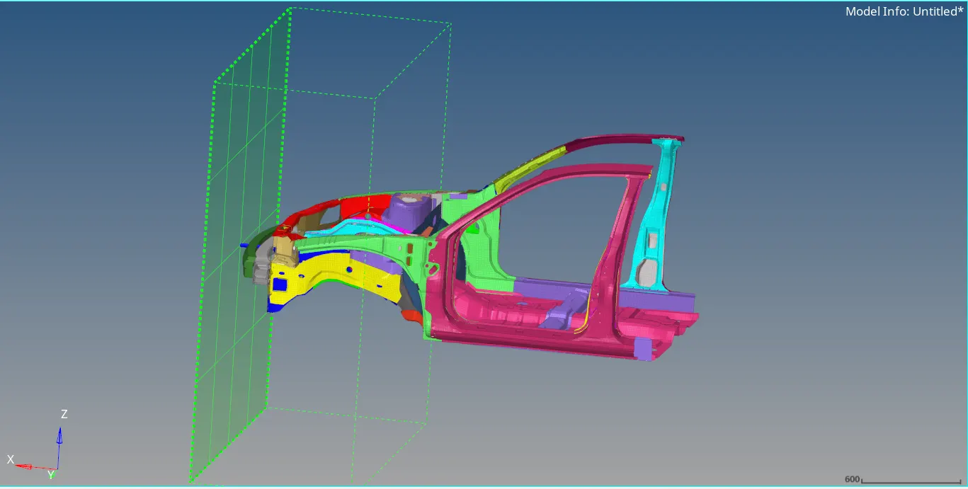
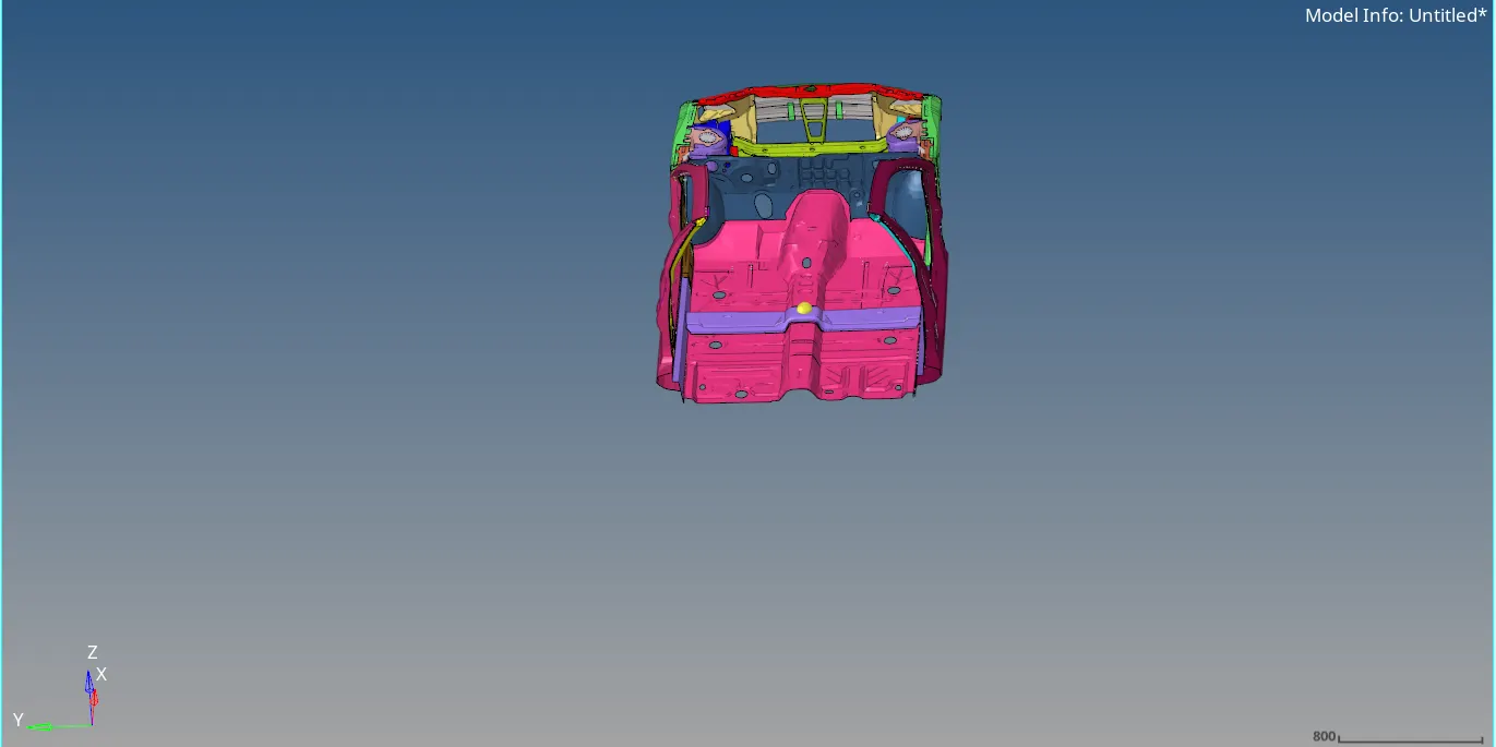
- Create a Rigid wall at the correct location with Dsearch = 1000 as shown below.
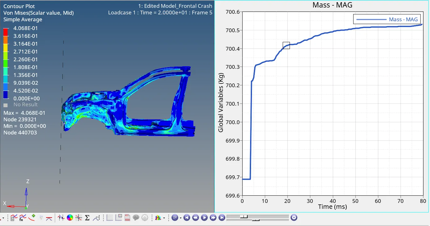
- Next, go to added masses and add new masses onto the floor section of the BIW so that the total mass of the BIW becomes 700 kg and the cog comes along the length of the driver seating position. In this case, the following masses have been added to the section
The cog now comes at the following location which is ideal for us. (node)
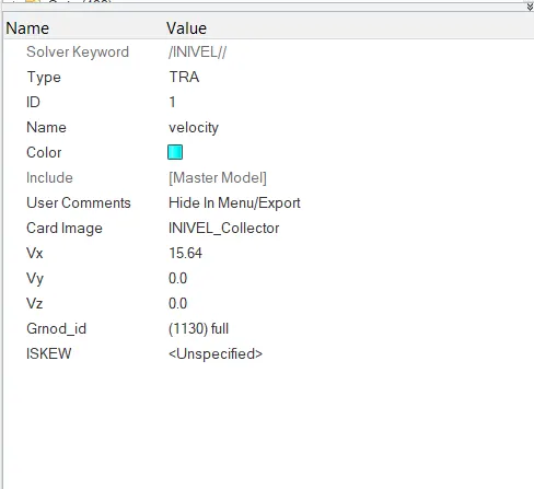
- Create load collector-->inivel-->15.64m/s in the x direction and select all nodes to apply this velocity to.
- Next, go to the model checker and run the errors and warnings.
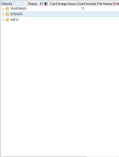
As long as there are no errors we can run the simulation without a problem.
- Next go to solver browser-->engine keywords-->DT/NODA , keep Tmin as 0.0005, Tscale = 0.67 and select CST_0 option so that timestep does not go below 0.5.
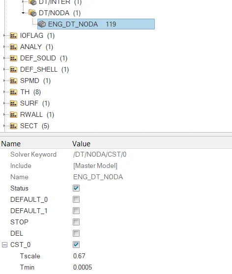
Do the same for DT/INTER as well so that the same procedure is followed.
Setting up Output Requests: Next, we will set up sections at the following nodal locations as requested.
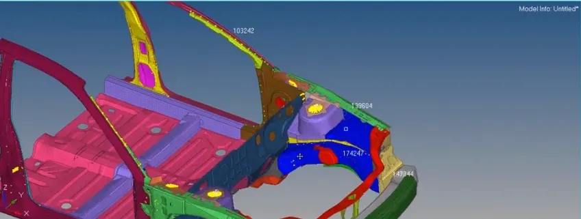
We will create sections by Create-->cross section-->select base node-->select direction of orientation and clicking create. If the correct elements and nodes do not get selected by this we will rectify them manually by going to sets and modifying the set of nodes and elements.
We have created 5 sections as shown below. They are at the following locations.
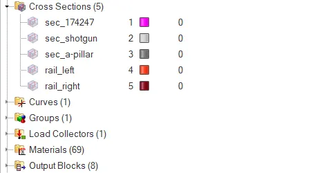
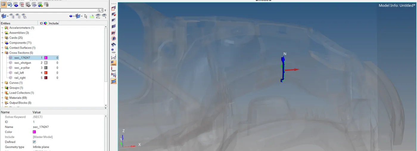
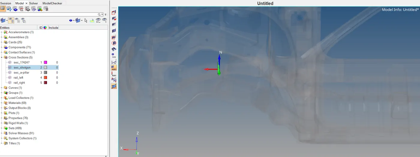
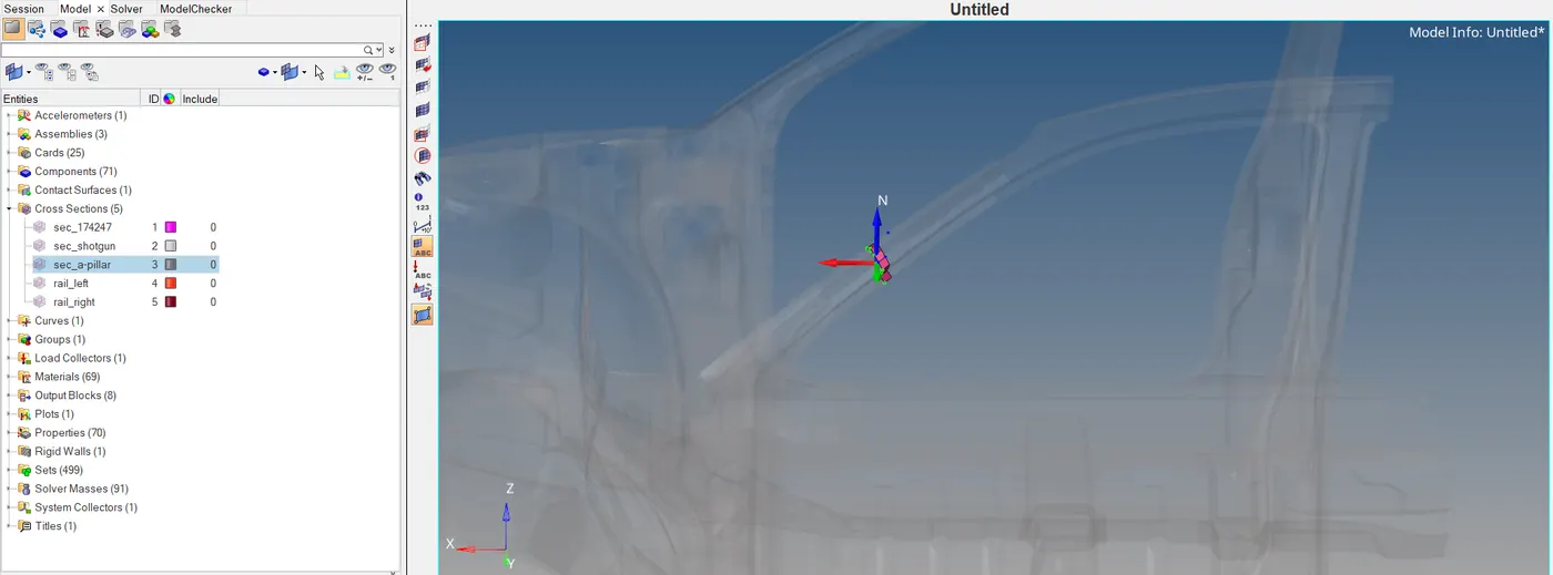
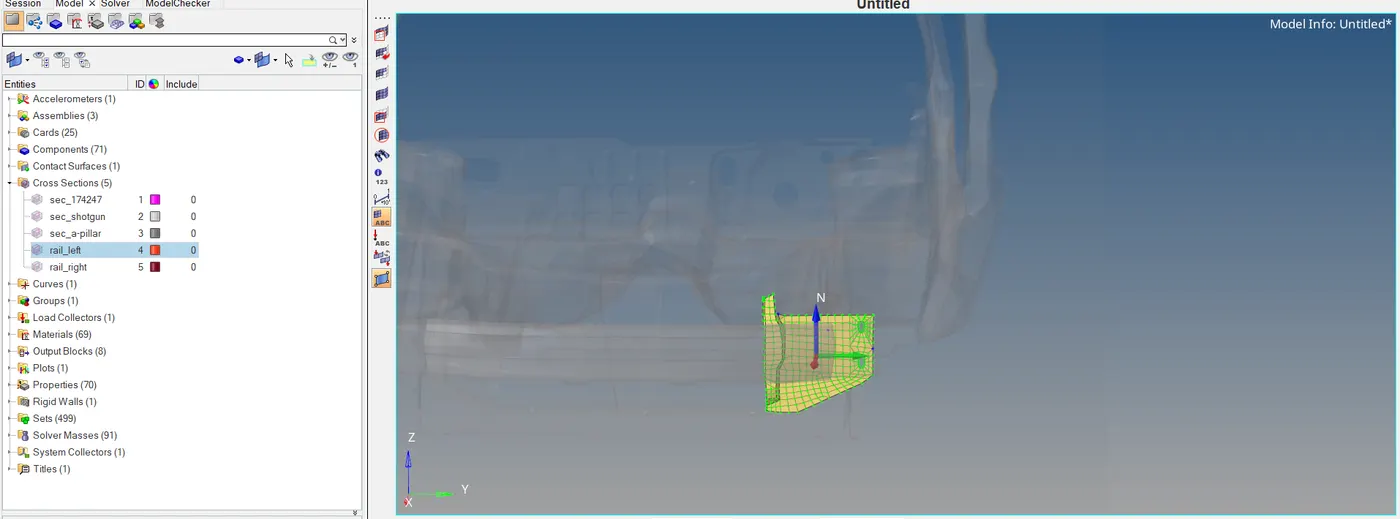
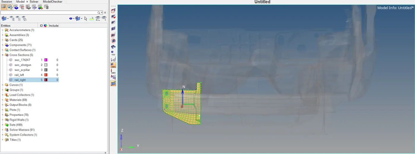
After this, add all the sections to separate output requests with DEF selected to get all the velocities and accels.
Next, we will create an accelerometer at the base of B-pillar as shown. Go to create-->accelerometer-->select node-->create
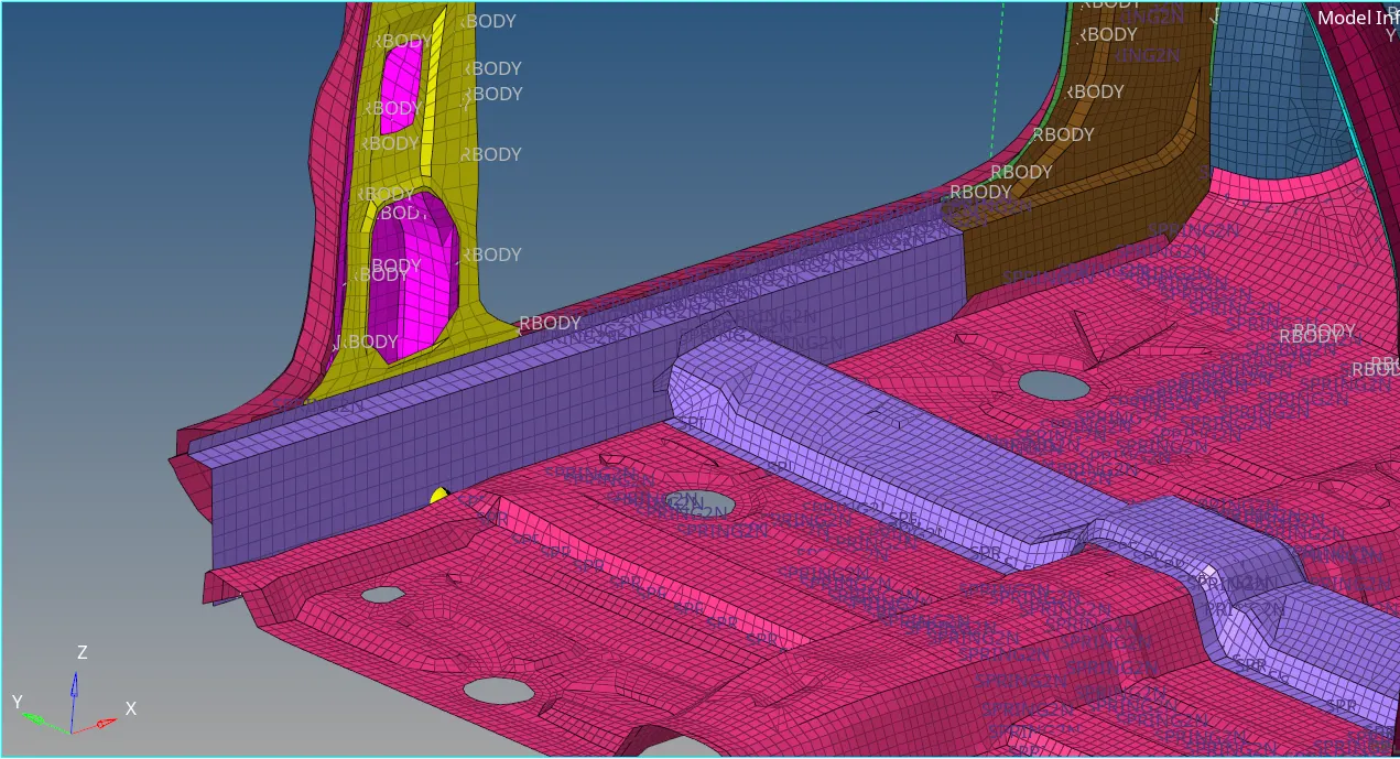
After this, add it to an output request with 3 variables selected to get accel in X, Y & Z respectively.
- Next, to measure intrusion we will measure the displacement of the 2 nodes 66695 & 66244 respectively.
We will create a local co-ordinate system a bit further dwon from those two nodes and measure their displacement ensuring the crash with respect to the local co-ordinate system. First, create SKEW/MOV in the solver browser as follows.
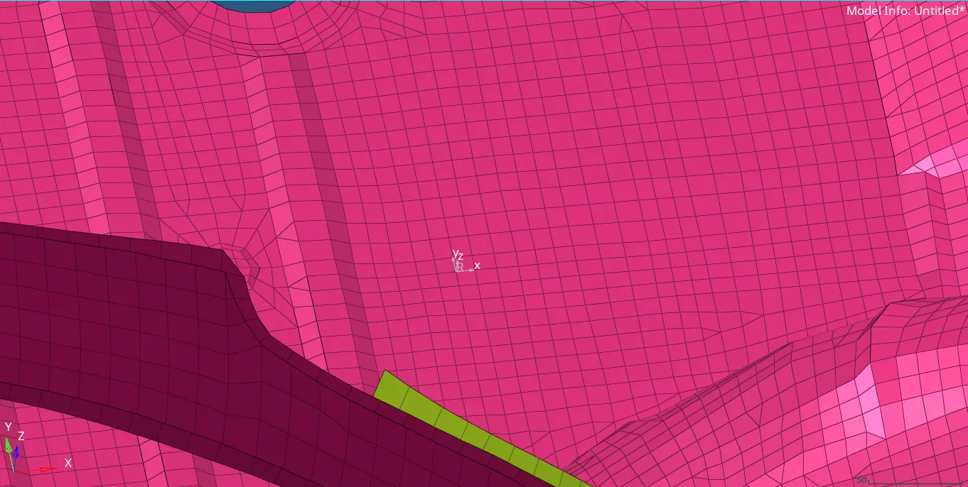
Next create output request TH/NODE, select both the nodes and select the skew id with respect to which it must be measured.
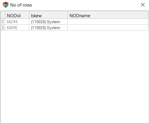
Select displacement to be measured as follows.
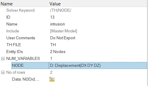
Run the simulation.
POST-PROCESSING :
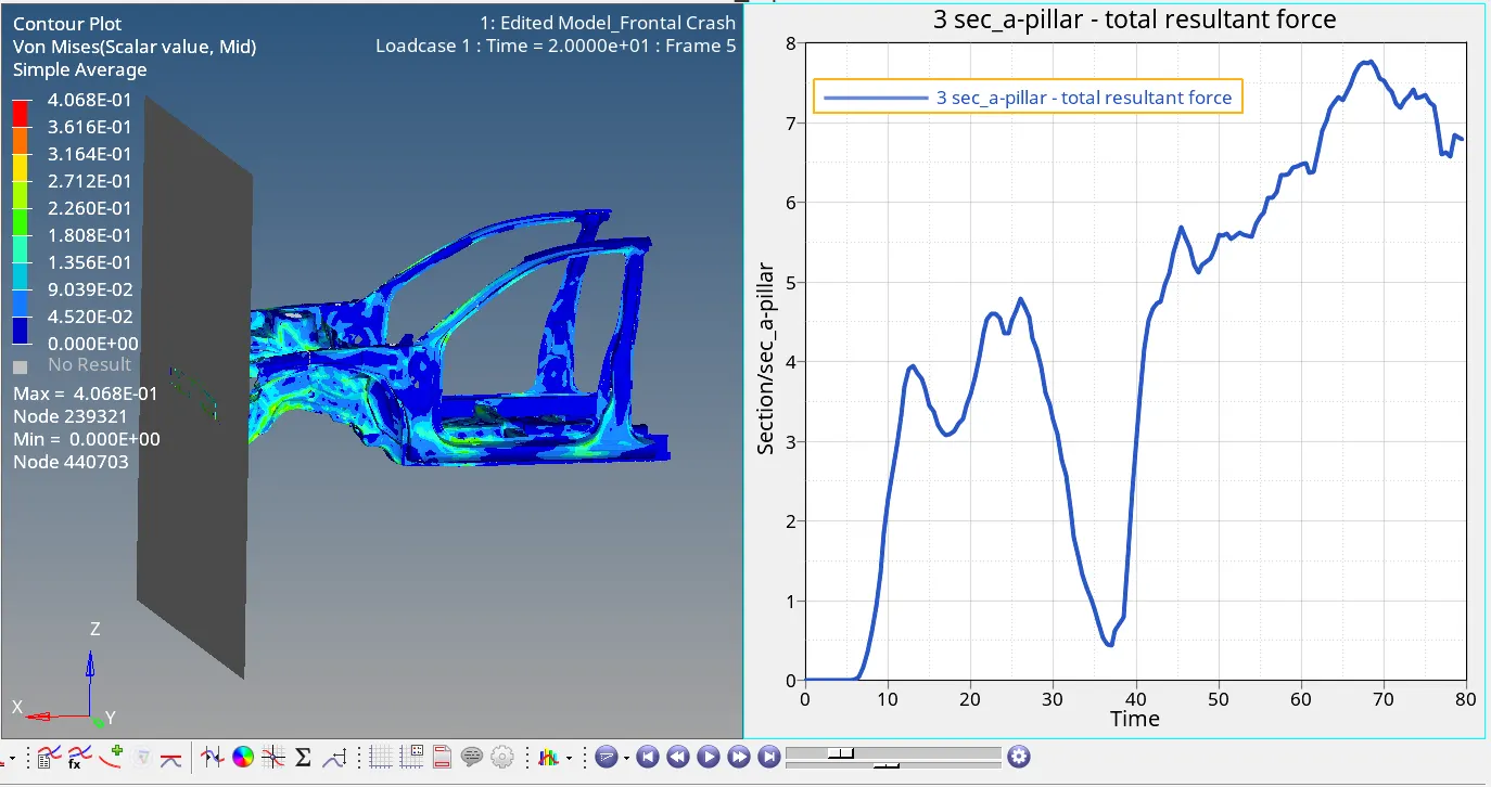
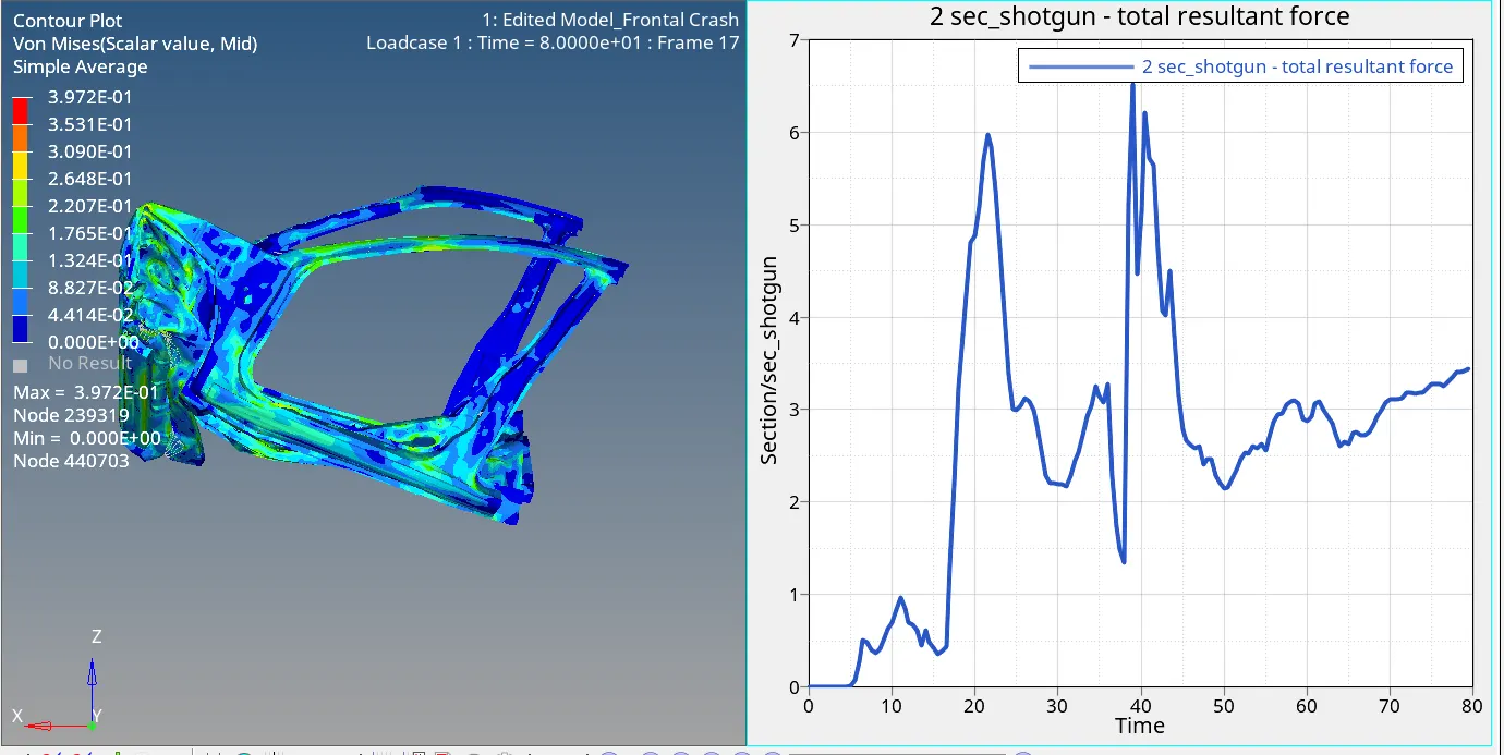
We first see the forces acting on the sections that we created as follows.
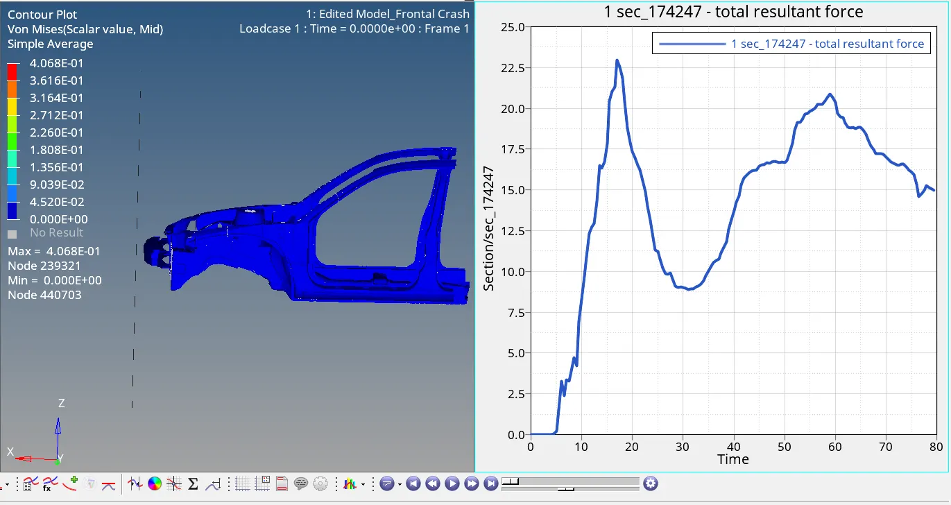
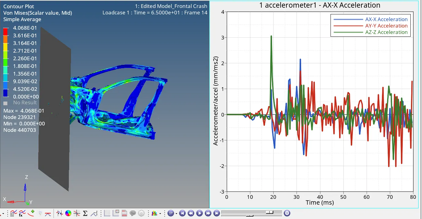
The accelerations received on the accelerometer are as follows:
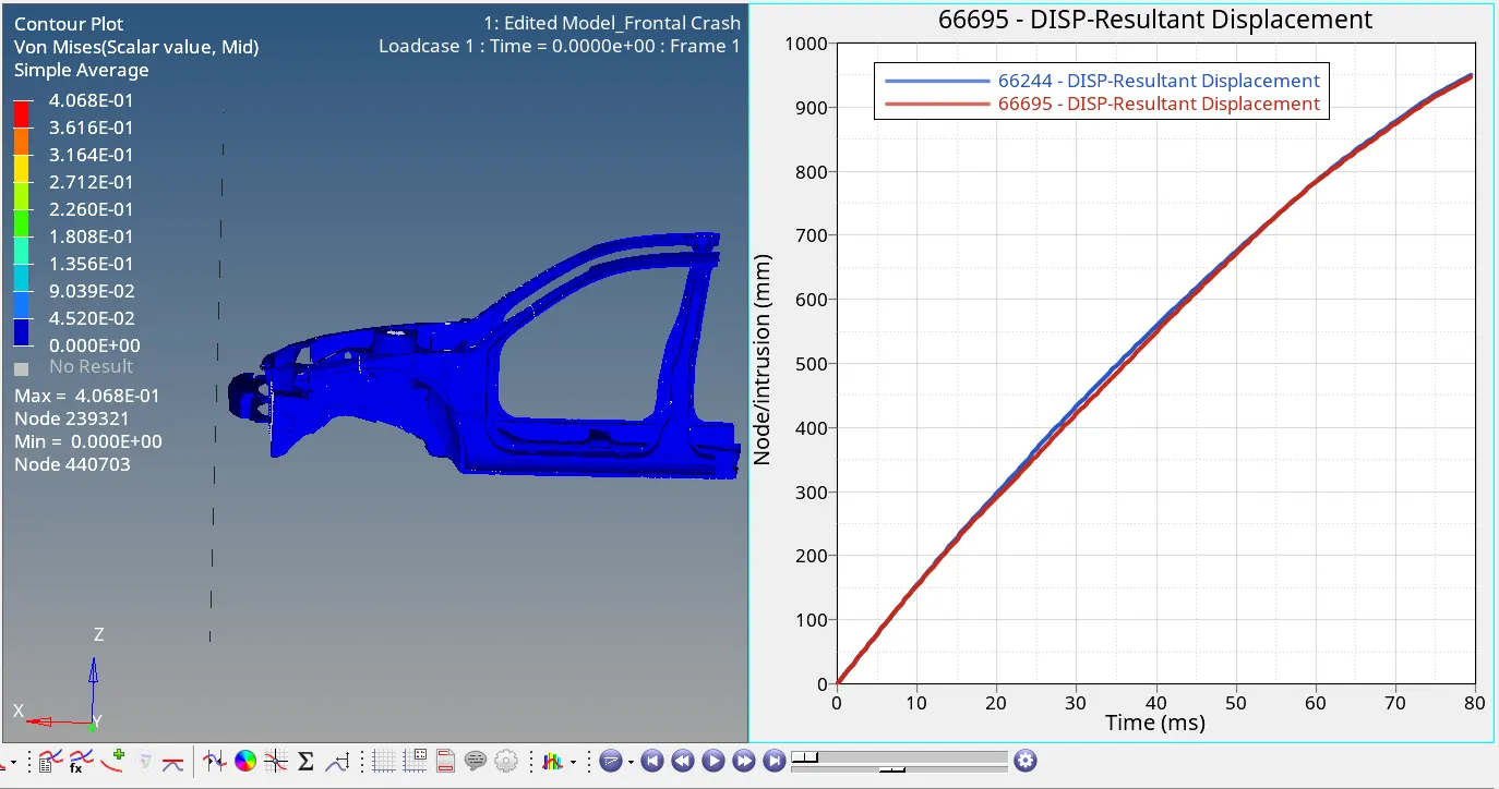
The intrusions in the foot pedal increase linearly as the simulation progress as we can see below :
Crash animation:
Stress
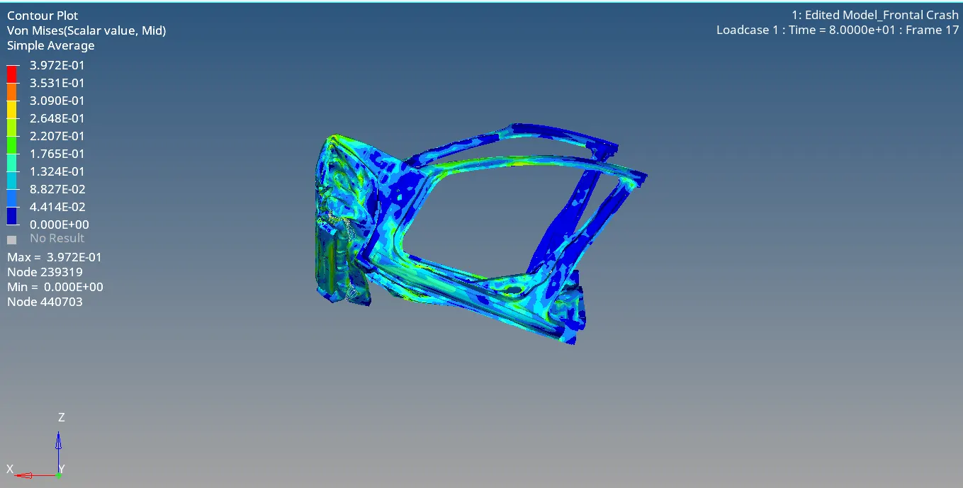
Upon crashing the car body undergoes torsion about the x-axis as we can see from this angle. This may be due to imbalances in the cog y co-ordinate or due to some other mass imbalances or asymmetry in the structure about x-axis. The peak stress is noted at 0.4068 Gpa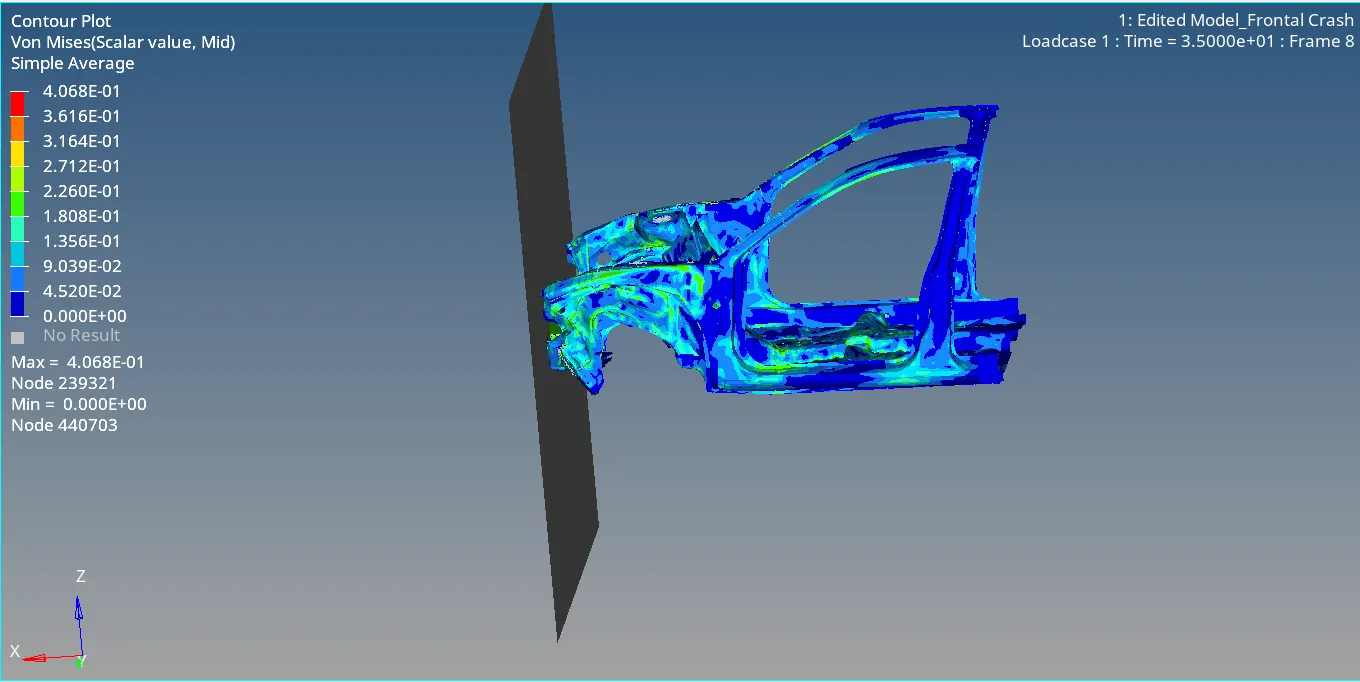
As we can see from the simulation, the bumper is the first to compress into the wall and get deformed. After that, the engine compartment gets compressed absorbing a lot of the energy. It forms the crumple zone so that minimum forces are transmitted to the passenger cabin so that the occupants can remain safe in the event of a crash.
Hourglass Energy:
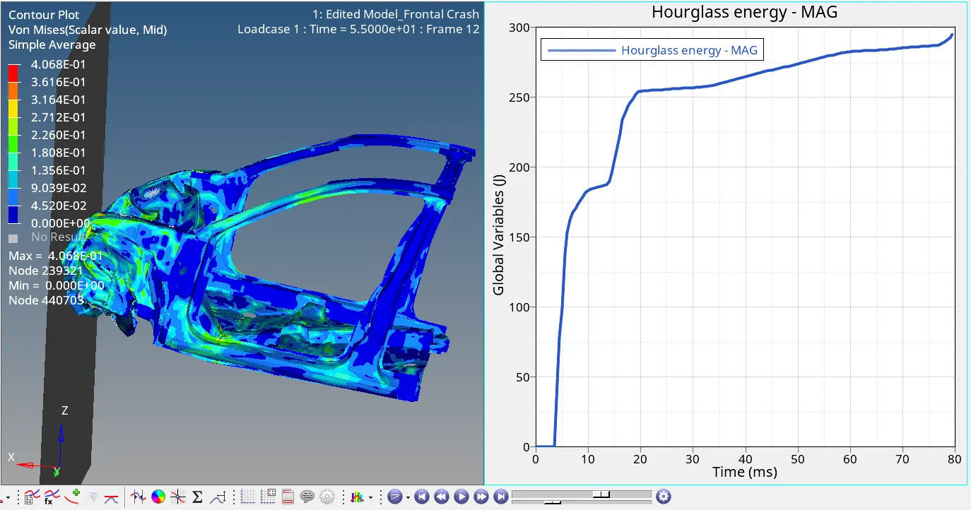
There is hourglass energy formation due to loss of total energy but the amount of Hourglass energy formation is minimum and well within the tolerance limits.
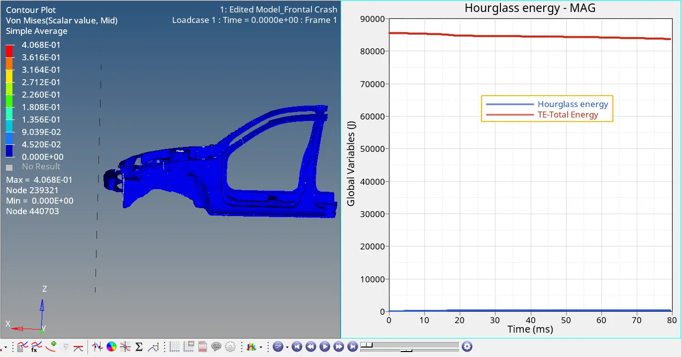
Total translational energy:
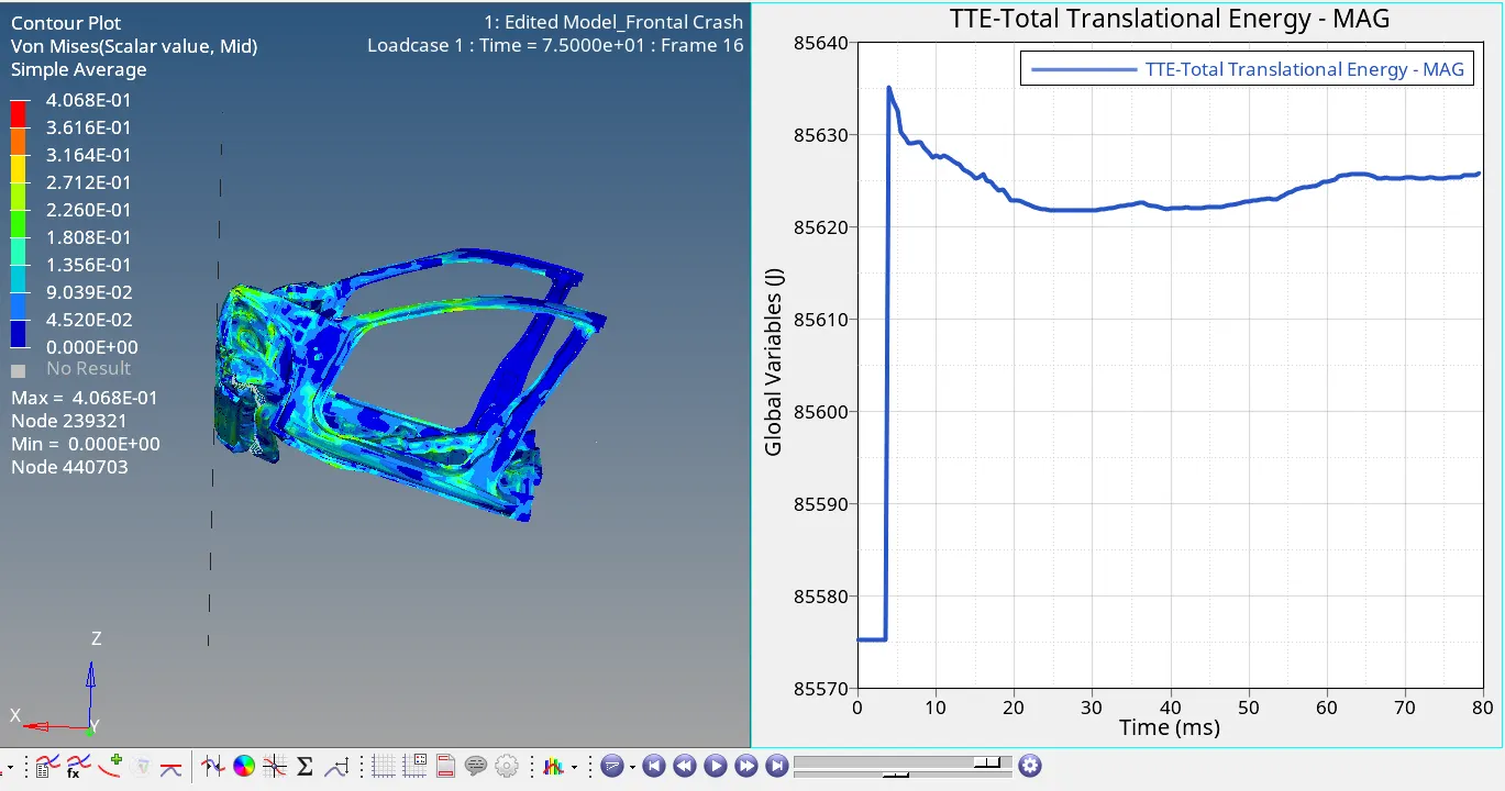
The total translational energy remains fairly constant throughout the simulation and varies by just a small amount.
Kinetic energy v/s Internal Energy:
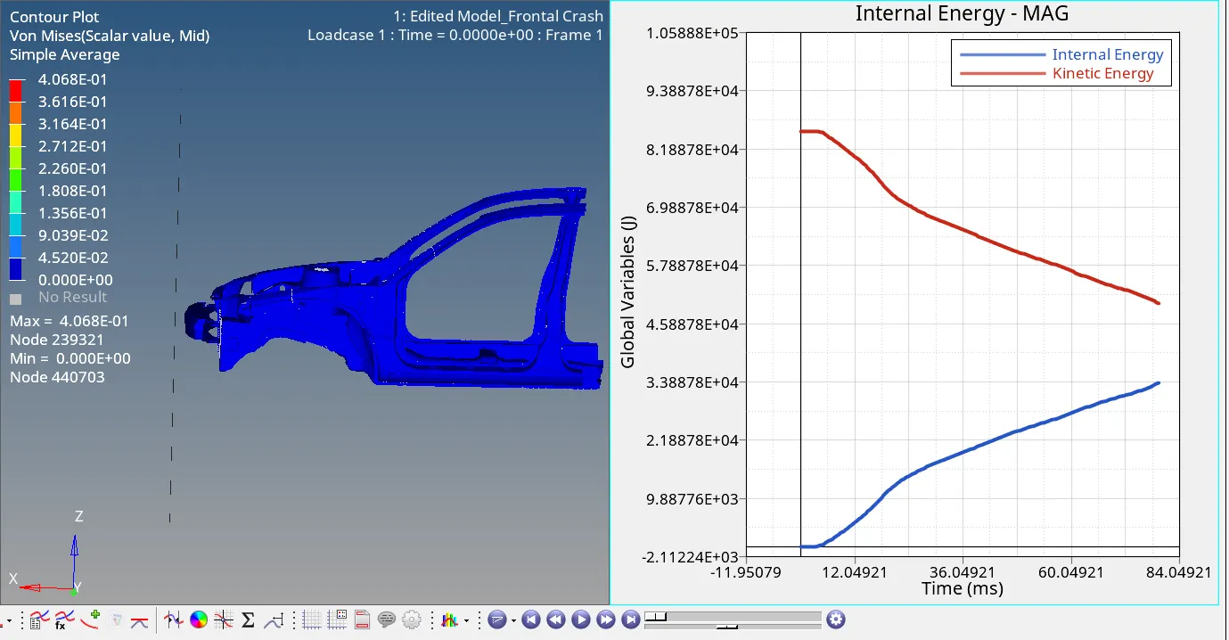
As this is an energy absorption simulation all the loss in kinetic energy directly translated to the increase in internal energy as is evident in the similar nature of the graphs here. This indicates that the energy error is minimum since the loss of KE is almost exactly equal to the gain in IE.
Contact Energy:
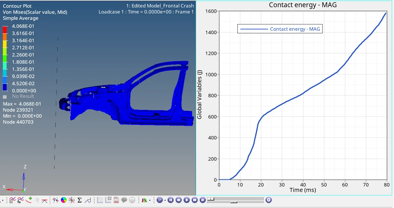
As we can see there is some amount of contact energy getting created as well as the simulation goes on. This increase in contact energy is directly proportional to the loss of total energy as shown below:
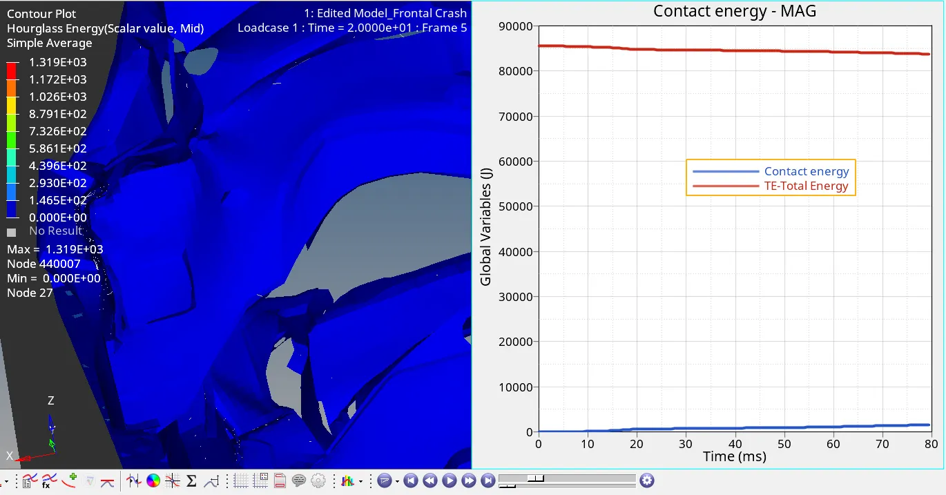
However, the total contact energy is around 2.1% of the total energy and so it is within the tolerance limit of 5%. Due to this drop in total energy, there is hourglass energy formation as well which is shown above.
Engine.out file
Energy error
If we look in the engine .out file we see a peak energy error of -2.1% as predicted.
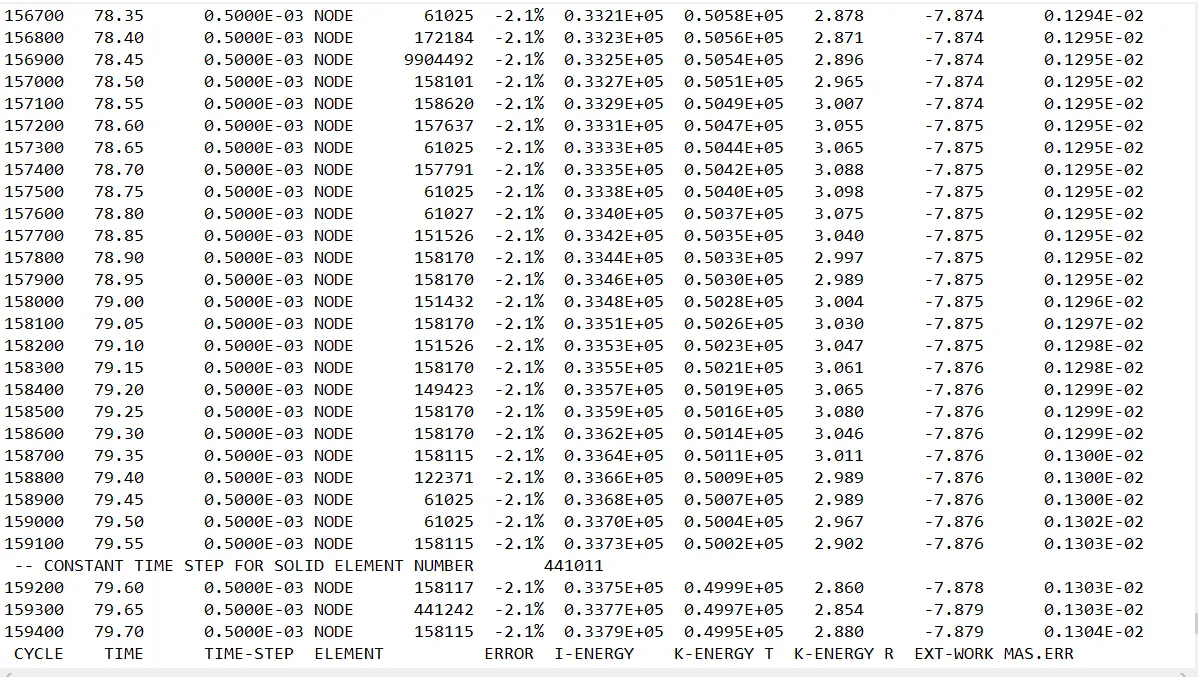
Mass error: The mass error reaches a peak value of 0.13% which is within the 1% tolerance limit that we must follow for mass error.
Timestep: Throughout the timestep, we can see that a minimum timestep of 0.5 microseconds has been maintained.
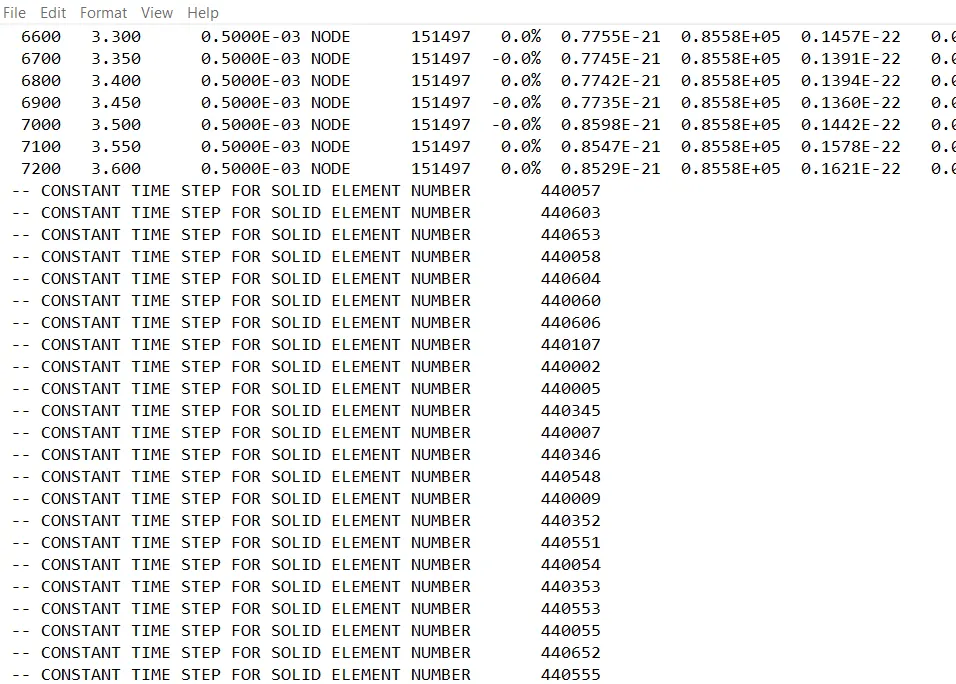
In certain sections, if the timestep is found to be going beneath that value it switches over to a small strain formulation and follows a constant timestep which we selected in DT/NODA-->CST_0. As we can see above the following elements were found to violate the minimum timestep so the processor took corrective action to maintain the speed of the simulation and avoid unnecessary calculations.
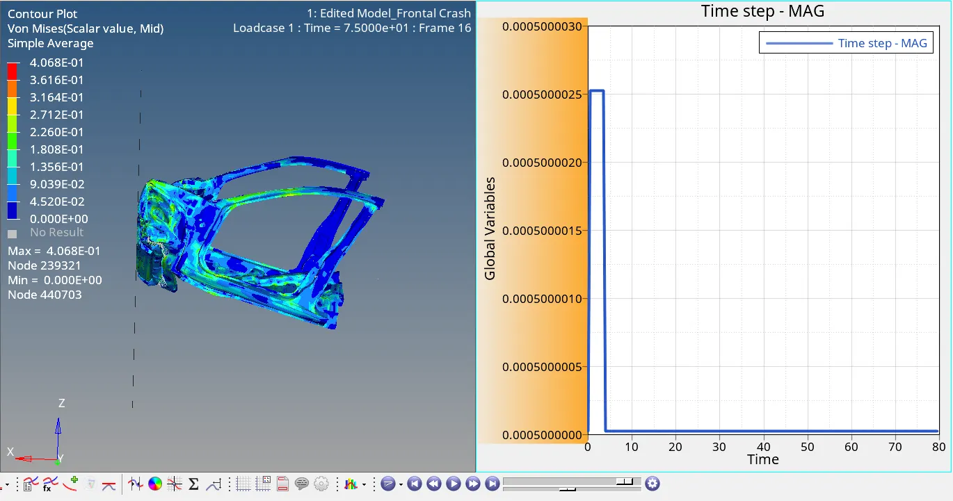
As we can see the graph for timestep is pretty linear and varies by a very small margin right at the beginning to account for mass addition at the beginning after which it remains nearly constant throughout the rest of the simulation.
Errors: The energy errors although they are within tolerable limits they could be further improved by reducing the contact energy of the simulation. This could be done by adding further definition to the contacts by adding a type 11 contact as well to account for edge-to-edge penetrations. This will in turn prevent the hourglass energy formation as well and make the simulation more accurate.
Conclusion: The following simulation has been run according to the required conditions and the required outputs have been obtained.