Project 1 - Parsing NASA thermodynamic data
1.AIM:
- To write a function that extracts the 14 temperature co-efficients and calculates properties like molecular weight, enthalpy, entropy, and specific heats for all the species in the given data file.
- To plot and save enthalpy, entropy, and specific heats for the local temperature range specific for each species and save those plots into seperate folders.
2.GOVERNING EQUATIONS:
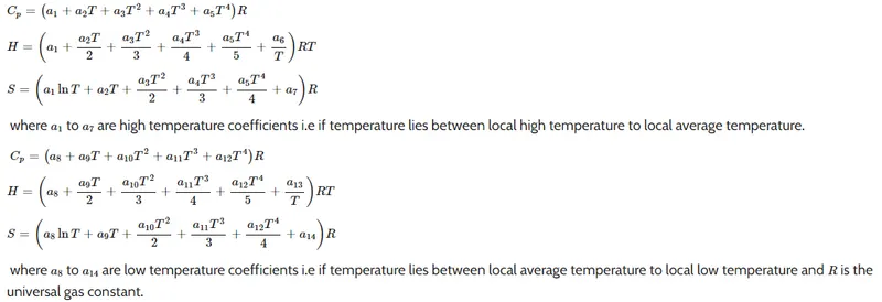
NASA came up with polynomials that can be used to evaluate thermodynamic properties such as Cp,H,S. These polynomials are given by
3.OBJECTIVES OF THE PROJECT:
- To extract the 14 coefficients and calculate the enthalpy, entropy and specific heats for all the species in the data file.
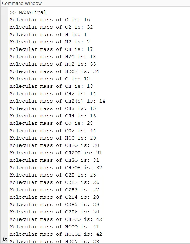
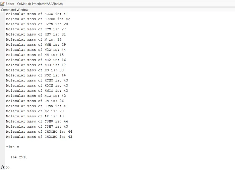
- To calculate the molecular weight of each species and display it in the command window.
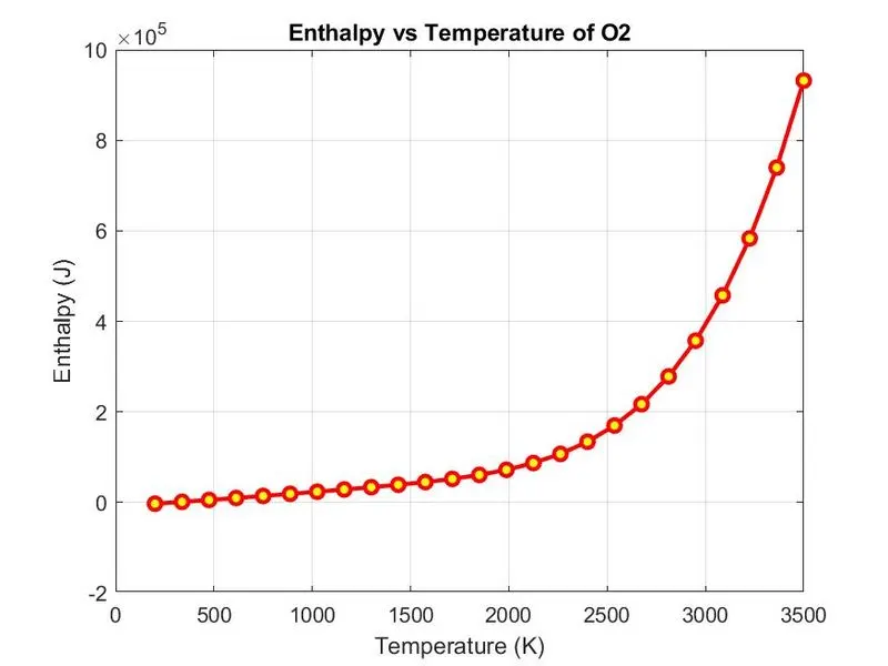
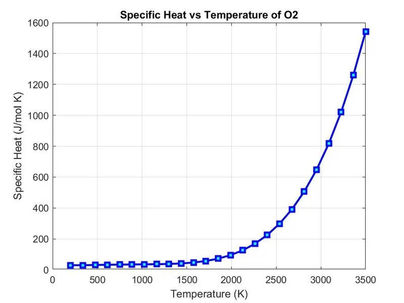
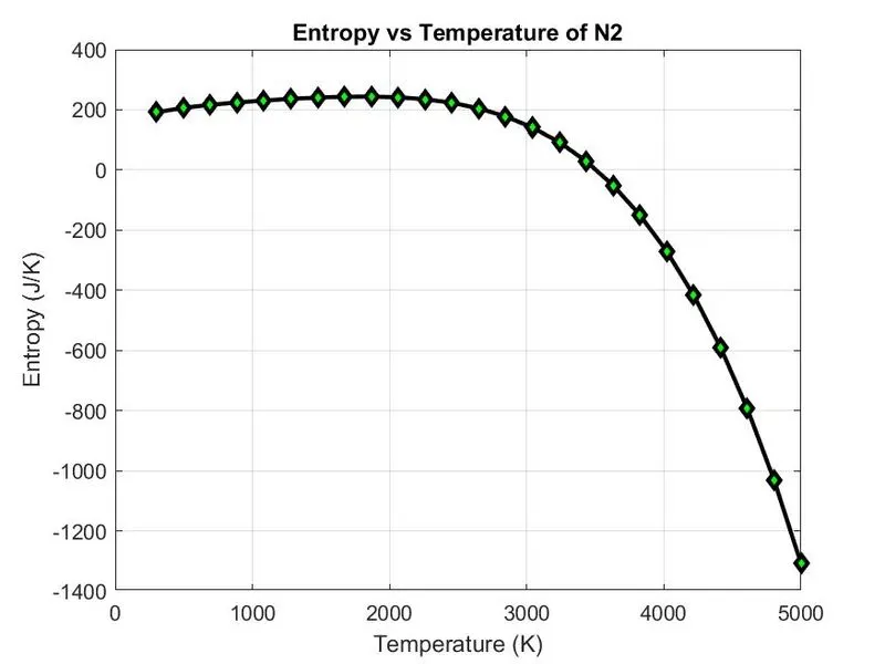
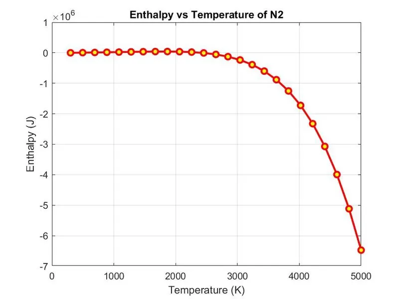
- To plot the Specific Heat, Enthalpy and Entropy for the local temperature range (low temperature:high temperature) specific for each species.
- To save the plots as images with appropriate names and dump them in separate folders for each species with a suitable name. (All these should be generated automatically)
- The main program should just take the THERMO.dat file as an input and generate Cp, H and S plots.
4.BODY OF THE PROJECT:
- Open the file using fgetl and read it using r.
- The fgetl command returns a character vector in the line. If the file is empty and contains only the end-of-file marker, fgetl returns a numeric value.
- The strsplit(A) command splits at whitespace. A whitespace character is equivalent to any sequence in the set {' ' 'n' 'f' 'r' 't' 'v'}.
- If str has consecutive whitespace characters, then strsplit treats them as one whitespace.
- The global temperatures are obtained in the form of strings from the line and converted into numerical values using str2double.
- The comments which are futile are also included in the code.
- Create a for loop i for data generation of all 53 species and their respective coefficients.
- Extract the first row of the file and convert it into an array using strsplit.
- Determine the local temperatures according to the position they are situated in.
- For coefficients, determine the position of exponent 'E' as a reference point and calculate subsequent values using the preceding one.
- Define the local temperature range for the plot and compute Cp, H, and S according to their respective ranges as defined in the problem.
- The mkdir command creates a folder in the given directory for the species.
- Create a for loop j for calculating Cp, H and S according to the local temperature ranges.
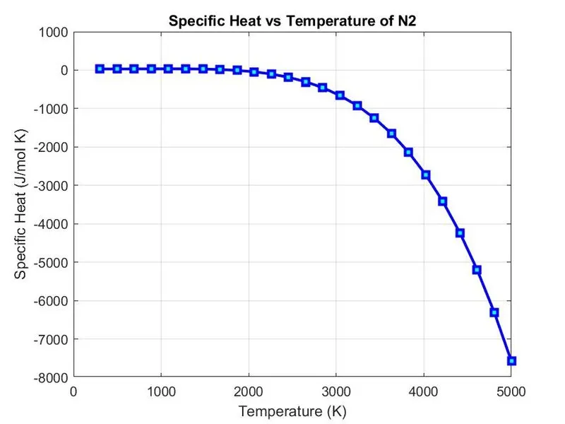
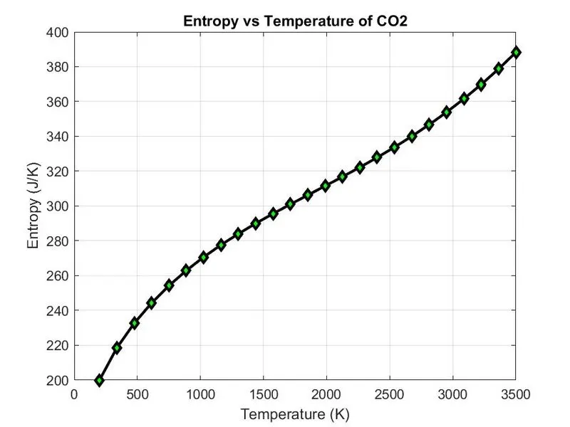
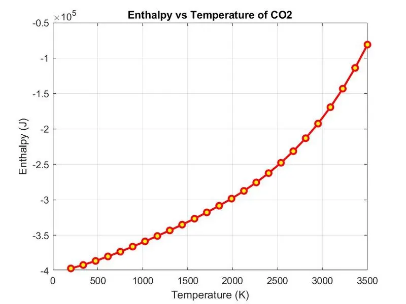
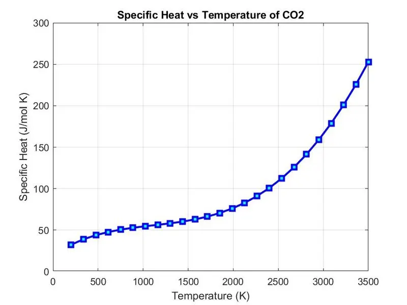
- Plots are plotted for Cp, H and S versus temperature.
- The directory is accessed as in step 11 and cd is used to change the current folder to a new folder.
- Plots are saved individually in the directory folders using saveas.
- Again move out of the folder one time to access the molecular_mass file and calculate it using the function as below.
- Terminate the file using fclose and operation.
- An explanation for the function is given below;
In the given file, the species are made up of the common individual elements H, C, O, N and A.
- Assign the atomic weight of the elements in an array respectively.
- For loop i takes the species as performed in the main program whereas the second loop j returns elements of the species.
- Compare both strings (specie name and element index) using strcmp; if they are equal it returns the MW accordingly.
- If the index exceeds 1 molecule, the molecular mass MW is the summation of previous molecular mass and (n-1) times the atomic weight.
Code: The MATLAB program to plot the P-V diagram is shown below.
% Program to parse NASA thermodynamic data file.

tic
file = fopen('THERMO.dat','r');    % Opening the file
header = fgetl(file);    % Extracting the title

temp = fgetl(file);     % Temperature
temp_array = strsplit(temp,' ');    % Converting into array

% Defining global temperatures from the array
global_low = str2double(temp_array{2});
global_mid = str2double(temp_array{3});
global_high = str2double(temp_array{4});

% Comments
c1 = fgetl(file);
c2 = fgetl(file);
c3 = fgetl(file);

% Reading the species and related data
for i = 1:53
    specie_data = fgetl(file);
    x = strsplit(specie_data,' ');      % Converting into array
    specie_name = x{1};     % Maximum specie name size
    y = length(x);      % Size of x

    % Defining local temperatures from the array
    local_low = str2double(x{y-3});
    local_mid = str2double(x{y-1});
    local_high = str2double(x{y-2});

    % Coefficients
    line1 = fgetl(file);
    L1 = strfind(line1,'E');
    a1 = str2double(line1(1:(L1(1)+3)));
    a2 = str2double(line1(L1(1)+4:(L1(2)+3)));
    a3 = str2double(line1(L1(2)+4:(L1(3)+3)));
    a4 = str2double(line1(L1(3)+4:(L1(4)+3)));
    a5 = str2double(line1(L1(4)+4:(L1(5)+3)));

    line2 = fgetl(file);
    L2 = strfind(line2,'E');
    a6 = str2double(line2(1:(L2(1)+3)));
    a7 = str2double(line2(L2(1)+4:(L2(2)+3)));
    a8 = str2double(line2(L2(2)+4:(L2(3)+3)));
    a9 = str2double(line2(L2(3)+4:(L2(4)+3)));
    a10 = str2double(line2(L2(4)+4:(L2(5)+3)));

    line3 = fgetl(file);
    L3 = strfind(line3,'E');
    a11 = str2double(line3(1:(L3(1)+3)));
    a12 = str2double(line3(L3(1)+4:(L3(2)+3)));
    a13 = str2double(line3(L3(2)+4:(L3(3)+3)));
    a14 = str2double(line3(L3(3)+4:(L3(4)+3)));

    % Inputs:
    T = linspace(local_low,local_high,25);
    R = 8.314;

    % Folder creation for species
    mkdir(['C:\Matlab Practice\Species\',specie_name])

    % Calculations
    for j = 1:length(T)
        if T >= local_mid
            Cp = R.*(a1 + a2.*(T) + a3.*(T.^2) + a4.*(T.^3) + a5.*(T.^4) + a6.*(T.^5));
            h = R.*(T).*(a1 + a2.*(T)./2 + a3.*(T.^2)./3 + a4.*(T.^3)./4 + a5.*(T.^4)./5 + a6./(T));
            S = R.*(a1.*log(T) + a2.*(T) + a3.*(T.^2)./2 + a4.*(T.^3)./3 + a5.*(T.^4)./4 + a7);
        else
            Cp = R.*(a8 + a9.*(T) + a10.*(T.^2) + a11.*(T.^3) + a12.*(T.^4));
            h = R.*T.*(a8 + a9.*(T)./2 + a10.*(T.^2)./3 + a11.*(T.^3)./4 + a12.*(T.^4)./5 + a13./(T));
            S = R.*(a8.*log(T) + a9.*(T) + a10.*(T.^2)./2 + a11.*(T.^3)./3 + a12.*(T.^4)./4 + a14);
        end
    end


% Plot:
figure(1)
plot(T,Cp,'-sb','markerfacecolor','c','linewidth',2)
xlabel('Temperature (K)')
ylabel('Specific Heat (J/mol K)')
title(sprintf('Specific Heat vs Temperature of %s',specie_name))
grid on

figure(2)
plot(T,h,'-or','markerfacecolor','y','linewidth',2)
xlabel('Temperature (K)')
ylabel('Enthalpy (J)')
title(sprintf('Enthalpy vs Temperature of %s',specie_name))
grid on

figure(3)
plot(T,S,'-dk','markerfacecolor','g','linewidth',2)
xlabel('Temperature (K)')
ylabel('Entropy (J/K)')
title(sprintf('Entropy vs Temperature of %s',specie_name))
grid on

cd(['C:\Matlab Practice\Species\',specie_name])     % Redirecting plots to the folders

% Saving the plots
saveas(1,'Specific Heat vs Temperature.jpg');
saveas(2,'Enthalpy vs Temperature.jpg');
saveas(3,'Entropy vs Temperature.jpg');

cd('C:\Matlab Practice\')      % Access the function file to get mol_weight mass

mol_weight(i) = molecular_mass(specie_name);

end

fclose(file);       % Closing the file
time = toc          % Total simulation time
Code for Function used:
function [MW] = molecular_mass(specie_name)

elements = ['H','C','N','O','A'];
atomic_weight = [1 12 14 16 40];

fprintf('Molecular mass of ')
fprintf(specie_name)
fprintf(' is: ')

MW = 0;
for i = 1:length(specie_name)
    for j = 1:length(elements)

       if strcmp(specie_name(i),elements(j))
           MW = MW + atomic_weight(j);
           position = j;
       end
    end

    n = str2double(specie_name(i));
    if n>1
        MW = MW + atomic_weight(position)*(n-1);
    end
end

fprintf('%d \n',MW);

end
5.OBSERVATION:
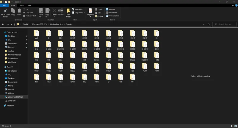
Folder for Species:
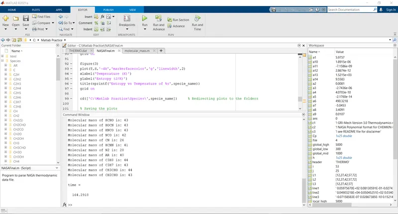
Screen Snip of Matlab Window:
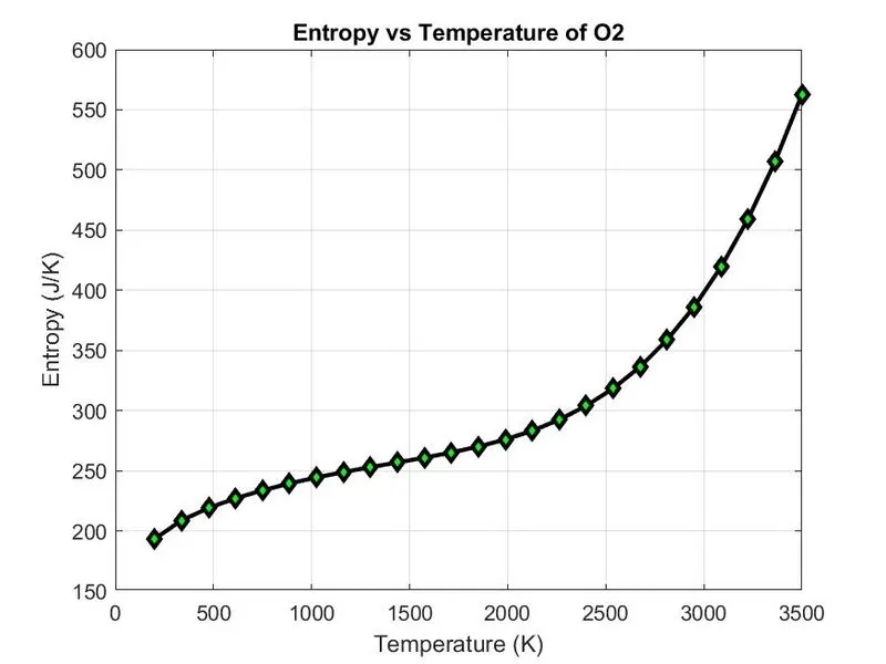
Outputs of O2,N2 and CO2:
Molecular weight of all species:
CONCLUSION:
- The project of Parsing Thermodynamic Data was successfully completed.
- The time taken for performing the operation was 164.2918 seconds.
REFERENCES: THERMO.DAT