Week 4.1 - Genetic Algorithm
1.AIM:
- To write a program on Matlab to optimise the stalagmite function and find the global maxima of the function.
- To explain the concept of Genetic Algorithm and the syntax for ga.
2.INTRODUCTION:
A Genetic Algorithm (GA) is a search-based optimization technique based on the principles of Genetics and Natural Selection. It is frequently used to find optimal or near-optimal solutions to difficult problems which otherwise would take a lifetime to solve. It is frequently used to solve optimization problems, in research, and in machine learning. GAs are a subset of a much larger branch of computation known as Evolutionary Computation. GAs were developed by John Holland and his students and colleagues at the University of Michigan, most notably David E. Goldberg, and have since been tried on various optimization problems with a high degree of success.
Genetic Algorithms are primarily used in optimization problems of various kinds, but they are frequently used in other application areas as well.
The areas in which Genetic Algorithms are frequently used are listed below.
- Optimization − Genetic Algorithms are most commonly used in optimization problems wherein we have to maximize or minimize a given objective function value under a given set of constraints.
- Economics − GAs are also used to characterize various economic models like the cobweb model, game theory equilibrium resolution, asset pricing, etc.
- Neural Networks − GAs are also used to train neural networks, particularly recurrent neural networks.
- Image Processing − GAs are used for various digital image processing (DIP) tasks as well as dense pixel matching.
Syntax for Genetic Algorithm
x = ga(fun,nvars)x = ga(fun,nvars,A,b)x = ga(fun,nvars,A,b,Aeq,beq)x = ga(fun,nvars,A,b,Aeq,beq,lb,ub)x = ga(fun,nvars,A,b,Aeq,beq,lb,ub,nonlcon)x = ga(fun,nvars,A,b,Aeq,beq,lb,ub,nonlcon,options)x = ga(fun,nvars,A,b,[],[],lb,ub,nonlcon,IntCon)x = ga(fun,nvars,A,b,[],[],lb,ub,nonlcon,IntCon,options)x = ga(problem)[x,fval] = ga(___)[x,fval,exitflag,output] = ga(___)[x,fval,exitflag,output,population,scores] = ga(___)x = ga(fun,nvars,A,b)x to fun, subject to the linear inequalities A*x ≤ b. ga evaluates the matrix product A*x as if x is transposed (A*x').
x = ga(fun,nvars,A,b,Aeq,beq)x to fun, subject to the linear equalities Aeq*x = beq and A*x ≤ b. (Set A=[] and b=[] if no linear inequalities exist.) ga evaluates the matrix product Aeq*x as if x is transposed (Aeq*x').
x = ga(fun,nvars,A,b,Aeq,beq,lb,ub)x, so that a solution is found in the range lb ≤ x ≤ ub. (Set Aeq=[] and beq=[] if no linear equalities exist.)
x = ga(fun,nvars,A,b,Aeq,beq,lb,ub,nonlcon)nonlcon. The function nonlcon accepts x and returns vectors C and Ceq, representing the nonlinear inequalities and equalities respectively. ga minimizes the fun such that C(x) ≤ 0 and Ceq(x) = 0. (Set lb=[] and ub=[] if no bounds exist.)
x = ga(fun,nvars,A,b,Aeq,beq,lb,ub,nonlcon,options)options. (Set nonlcon=[] if no nonlinear constraints exist.) Create options using optimoptions.
x = ga(fun,nvars,A,b,[],[],lb,ub,nonlcon,IntCon)x = ga(fun,nvars,A,b,[],[],lb,ub,nonlcon,IntCon,options)IntCon take integer values.
x = ga(problem)problem, a structure described in problem.
[, for any previous input arguments, also returns x,fval] = ga(___)fval, the value of the fitness function at x.
[ also returns x,fval,exitflag,output] = ga(___)exitflag, an integer identifying the reason the algorithm terminated, and output, a structure that contains output from each generation and other information about the performance of the algorithm.
[ also returns a matrix x,fval,exitflag,output,population,scores] = ga(___)population, whose rows are the final population, and a vector scores, the scores of the final population.
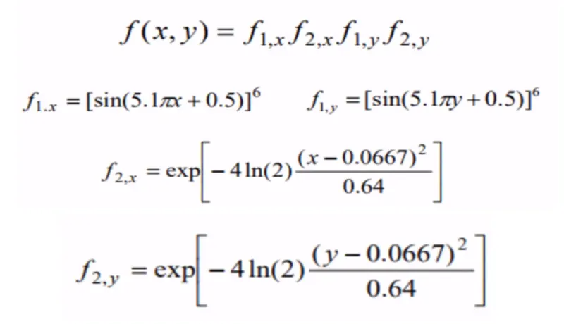
3.GOVERNING EQUATIONS:
4.OBJECTIVES OF THE PROJECT:
- Write a code in MATLAB to optimise the stalagmite function and find the global maxima of the function.
- To explain the concept of genetic algorithm and also explain the syntax for ga in MATLAB.
- To plot graphs for all 3 studies and for F maximum vs no. of iterations.
5.BODY OF THE PROJECT:
-
Firstly, a mesh is created using 'meshgrid' command from two input vectors 'x' and 'y' which will be acting as search space to find the maxima of the function.
-
The No of iterations 'limit' is defined by considering the no of iterations as 50,100,200.
-
The fitness of the function in each case is calculated.
-
The optimum value of the fitness function is evaluated in each iteration without considering the boundaries of x and y.
-
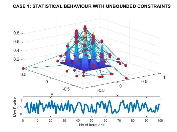
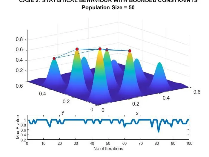
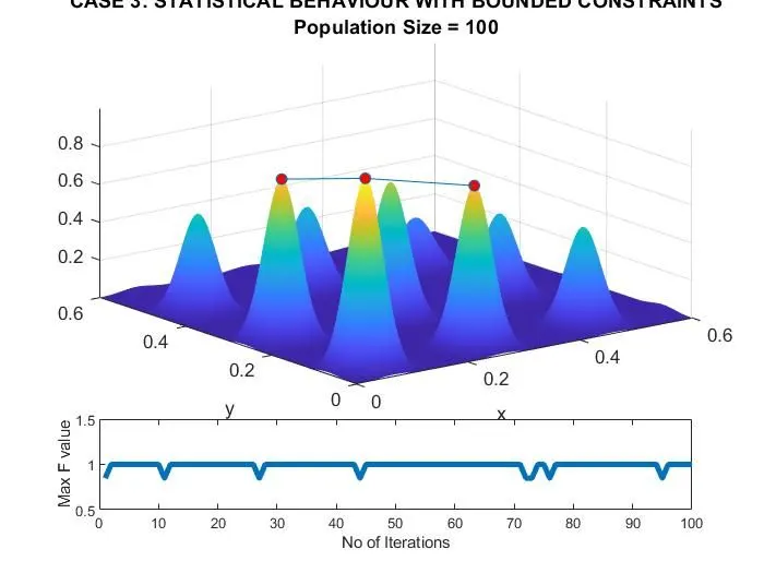
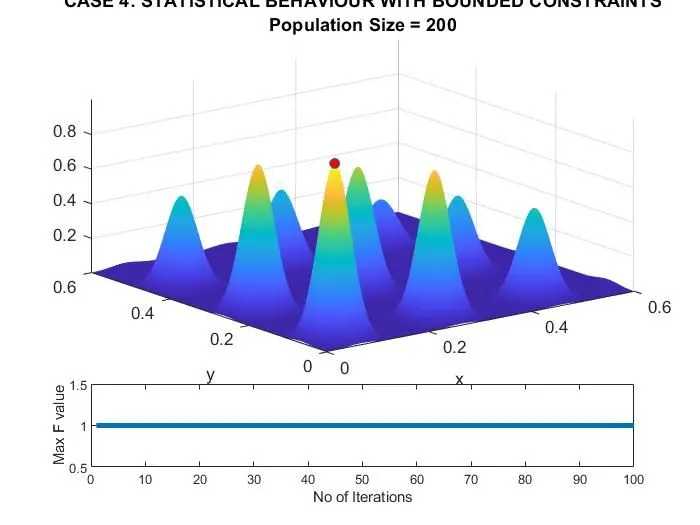
The stalagmite function is plotted using surf command and also optimum values obtained in each iteration are plotted onto the surface plot to check how the optimum values of the function are varying.
-
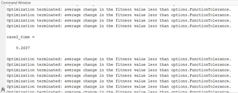
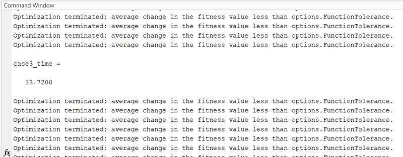
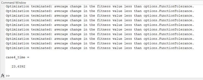
The 'tic' and 'toc' commands are used to evaluate the time taken for optimizing the function and the value is stored into case_time.
- The plot3 command is used to generate a 3D plot of x_out, y_out and optimum value of the function with the 'o' marker. The subplot command places these plots in a single window.
Code: The MATLAB program to plot the P-V diagram is shown below.
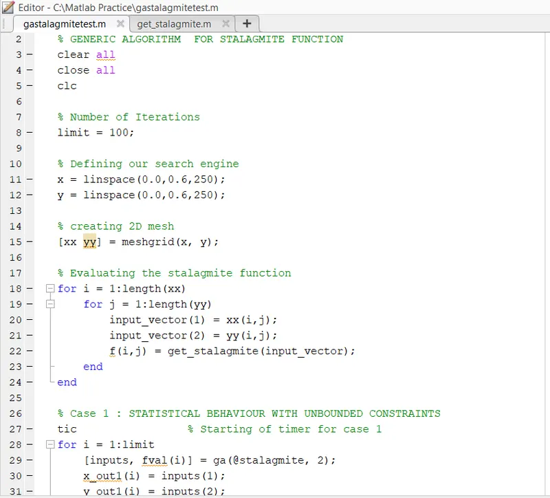
% GENERIC ALGORITHM  FOR STALAGMITE FUNCTION
clear all
close all
clc

% Number of Iterations
limit = 100;

% Defining our search engine
x = linspace(0.0,0.6,250);
y = linspace(0.0,0.6,250);

% creating 2D mesh
[xx yy] = meshgrid(x, y);

% Evaluating the stalagmite function
for i = 1:length(xx)
    for j = 1:length(yy)
        input_vector(1) = xx(i,j);
        input_vector(2) = yy(i,j);
        f(i,j) = get_stalagmite(input_vector);
    end
end

% Case 1 : STATISTICAL BEHAVIOUR WITH UNBOUNDED CONSTRAINTS
tic                 % Starting of timer for case 1
for i = 1:limit
    [inputs, fval(i)] = ga(@stalagmite, 2);
    x_out1(i) = inputs(1);
    y_out1(i) = inputs(2);
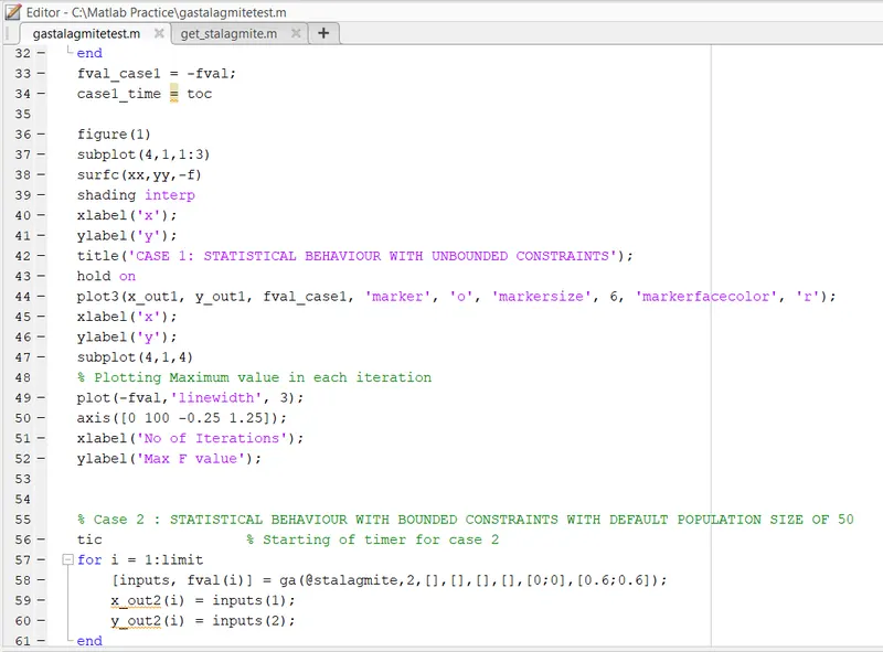
end
fval_case1 = -fval;
case1_time = toc

figure(1)
subplot(4,1,1:3)
surfc(xx,yy,-f)
shading interp
xlabel('x');
ylabel('y');
title('CASE 1: STATISTICAL BEHAVIOUR WITH UNBOUNDED CONSTRAINTS');
hold on
plot3(x_out1, y_out1, fval_case1, 'marker', 'o', 'markersize', 6, 'markerfacecolor', 'r');
xlabel('x');
ylabel('y');
subplot(4,1,4)
% Plotting Maximum value in each iteration
plot(-fval,'linewidth', 3);
axis([0 100 -0.25 1.25]);
xlabel('No of Iterations');
ylabel('Max F value');


% Case 2 : STATISTICAL BEHAVIOUR WITH BOUNDED CONSTRAINTS WITH DEFAULT POPULATION SIZE OF 50
tic                 % Starting of timer for case 2
for i = 1:limit
    [inputs, fval(i)] = ga(@stalagmite,2,[],[],[],[],[0;0],[0.6;0.6]);
    x_out2(i) = inputs(1);
    y_out2(i) = inputs(2);
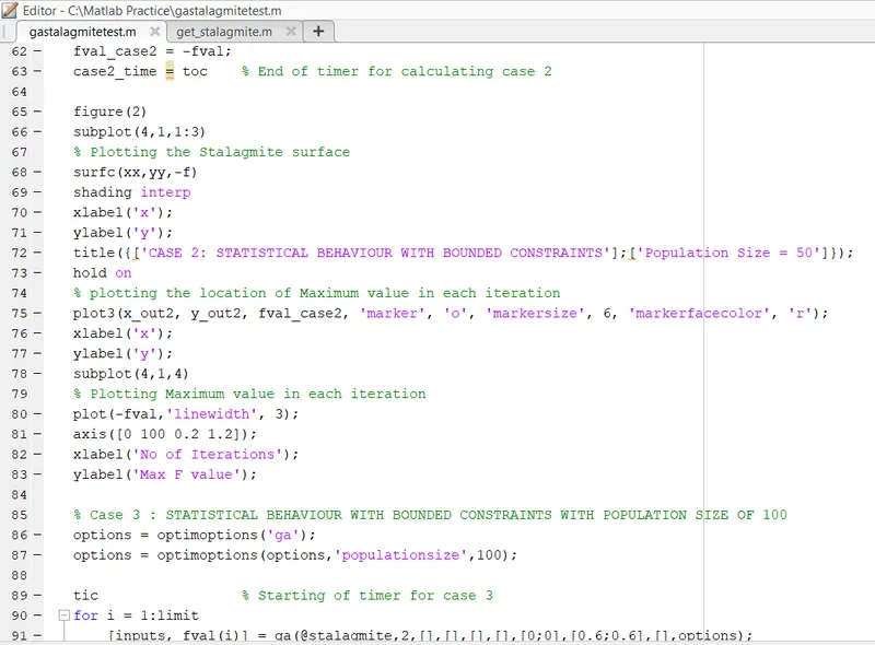
end
fval_case2 = -fval;
case2_time = toc    % End of timer for calculating case 2

figure(2)
subplot(4,1,1:3)
% Plotting the Stalagmite surface
surfc(xx,yy,-f)
shading interp
xlabel('x');
ylabel('y');
title({['CASE 2: STATISTICAL BEHAVIOUR WITH BOUNDED CONSTRAINTS'];['Population Size = 50']});
hold on
% plotting the location of Maximum value in each iteration
plot3(x_out2, y_out2, fval_case2, 'marker', 'o', 'markersize', 6, 'markerfacecolor', 'r');
xlabel('x');
ylabel('y');
subplot(4,1,4)
% Plotting Maximum value in each iteration
plot(-fval,'linewidth', 3);
axis([0 100 0.2 1.2]);
xlabel('No of Iterations');
ylabel('Max F value');

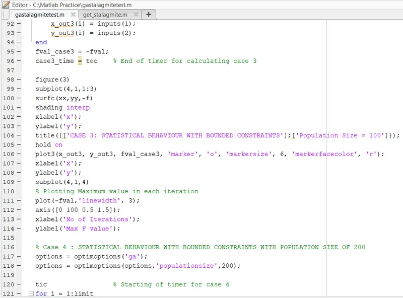
% Case 3 : STATISTICAL BEHAVIOUR WITH BOUNDED CONSTRAINTS WITH POPULATION SIZE OF 100
options = optimoptions('ga');
options = optimoptions(options,'populationsize',100);

tic                 % Starting of timer for case 3
for i = 1:limit
    [inputs, fval(i)] = ga(@stalagmite,2,[],[],[],[],[0;0],[0.6;0.6],[],options);
    x_out3(i) = inputs(1);
    y_out3(i) = inputs(2);
end
fval_case3 = -fval;
case3_time = toc    % End of timer for calculating case 3

figure(3)
subplot(4,1,1:3)
surfc(xx,yy,-f)
shading interp
xlabel('x');
ylabel('y');
title({['CASE 3: STATISTICAL BEHAVIOUR WITH BOUNDED CONSTRAINTS'];['Population Size = 100']});
hold on
plot3(x_out3, y_out3, fval_case3, 'marker', 'o', 'markersize', 6, 'markerfacecolor', 'r');
xlabel('x');
ylabel('y');
subplot(4,1,4)
% Plotting Maximum value in each iteration
plot(-fval,'linewidth', 3);
axis([0 100 0.5 1.5]);
xlabel('No of Iterations');
ylabel('Max F value');

% Case 4 : STATISTICAL BEHAVIOUR WITH BOUNDED CONSTRAINTS WITH POPULATION SIZE OF 200
options = optimoptions('ga');
options = optimoptions(options,'populationsize',200);

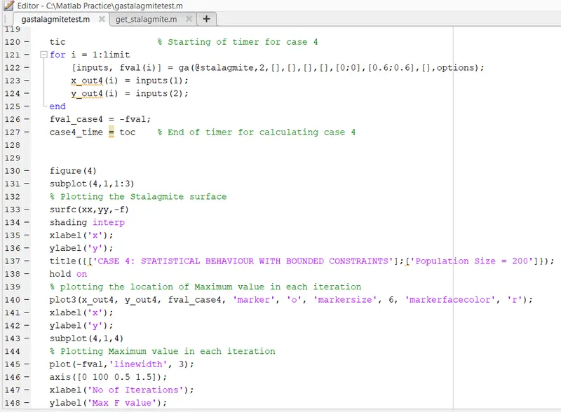
tic                 % Starting of timer for case 4
for i = 1:limit
    [inputs, fval(i)] = ga(@stalagmite,2,[],[],[],[],[0;0],[0.6;0.6],[],options);
    x_out4(i) = inputs(1);
    y_out4(i) = inputs(2);
end
fval_case4 = -fval;
case4_time = toc    % End of timer for calculating case 4


figure(4)
subplot(4,1,1:3)
% Plotting the Stalagmite surface
surfc(xx,yy,-f)
shading interp
xlabel('x');
ylabel('y');
title({['CASE 4: STATISTICAL BEHAVIOUR WITH BOUNDED CONSTRAINTS'];['Population Size = 200']});
hold on
% plotting the location of Maximum value in each iteration
plot3(x_out4, y_out4, fval_case4, 'marker', 'o', 'markersize', 6, 'markerfacecolor', 'r');
xlabel('x');
ylabel('y');
subplot(4,1,4)
% Plotting Maximum value in each iteration
plot(-fval,'linewidth', 3);
axis([0 100 0.5 1.5]);
xlabel('No of Iterations');
ylabel('Max F value');
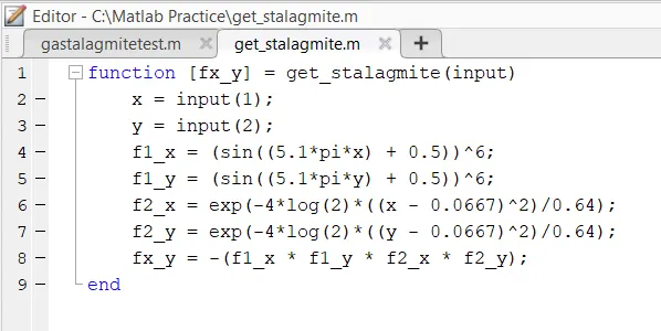
Code for Function used:
function [fx_y] = get_stalagmite(input)
    x = input(1);
    y = input(2);
    f1_x = (sin((5.1*pi*x) + 0.5))^6;
    f1_y = (sin((5.1*pi*y) + 0.5))^6;
    f2_x = exp(-4*log(2)*((x - 0.0667)^2)/0.64);
    f2_y = exp(-4*log(2)*((y - 0.0667)^2)/0.64);
    fx_y = -(f1_x * f1_y * f2_x * f2_y);
end
6.OBSERVATION:
Outputs of Editor:
Output of Function used:
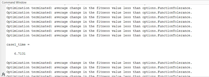
Outputs of Command Window:
Outputs of Graphs:
-
case1_time = 6.7131
-
case2_time = 9.2687
-
case3_time = 13.7200
-
case4_time = 23.6392
7.CONCLUSION:
The Genetic Algorithm challenge was successfully completed.
8.REFERENCES: