Week 3 - Solving second order ODEs

1.AIM: To write a program in Matlab to simulate the pendulum motion.

2.GOVERNING EQUATIONS:

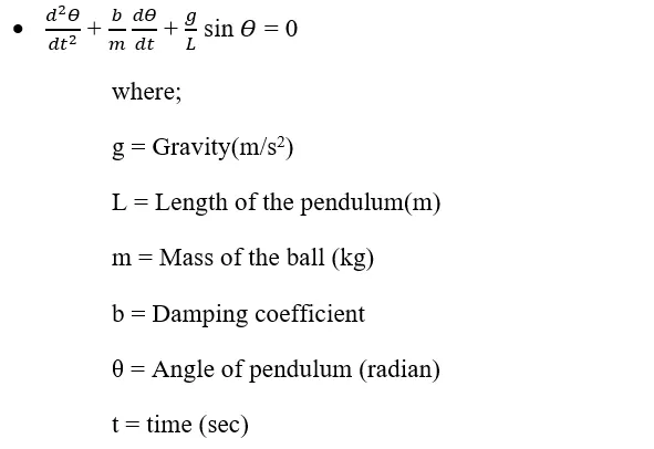
• The Ordinary Differential Equation (ODE) represents the equation of motion of a simple pendulum with damping as follows:

  

3.OBJECTIVES OF THE PROJECT:

• To write a program in Matlab to simulate the pendulum motion between 0-20 sec, for angular displacement=0, angular velocity=3 rad/sec at time t=0 using the following parameters:

L = 1 metre

m = 1 kg

b = 0.05

g = 9.81 m/s²

4.BODY OF THE PROJECT:

Explanation of Code used:

1. The input values are first stored.

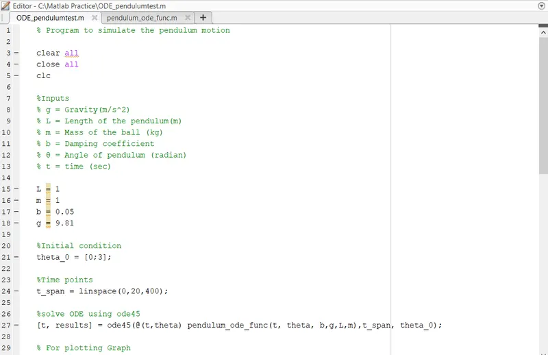
2. The ode45 function in Matlab is used to solve the ordinary differential equation with the input values and the solution will be stored in results.

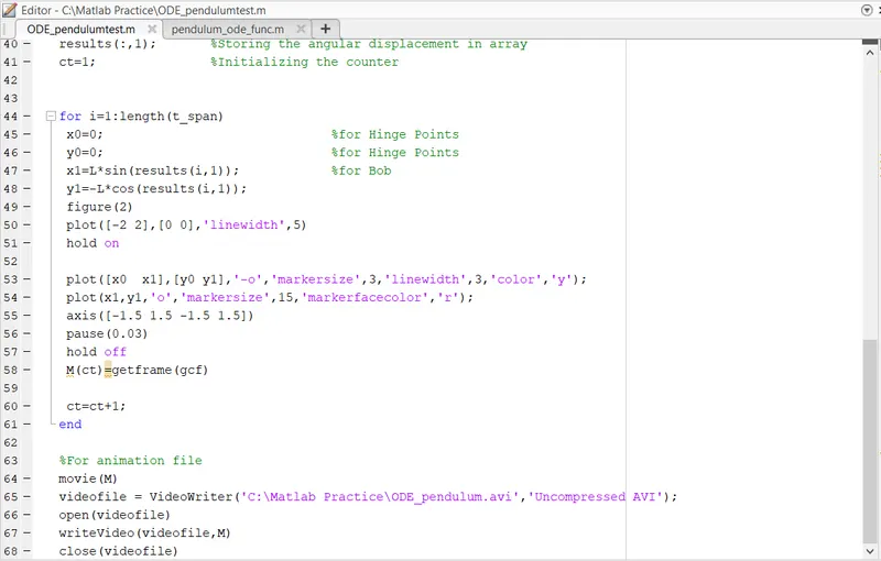
3. A for loop is used to capture the time and location of the pendulum.

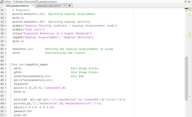
4. Finally, a graph is plotted using plot command and a video animation file is created by using the videofile command.

Code:

% Program to simulate the pendulum motion

clear all
close all
clc

%Inputs 
% g = Gravity(m/s^2)
% L = Length of the pendulum(m)
% m = Mass of the ball (kg)
% b = Damping coefficient
% θ = Angle of pendulum (radian)
% t = time (sec)

L = 1 
m = 1 
b = 0.05
g = 9.81 

%Initial condition
theta_0 = [0;3]; 

%Time points
t_span = linspace(0,20,400);

%solve ODE using ode45
[t, results] = ode45(@(t,theta) pendulum_ode_func(t, theta, b,g,L,m),t_span, theta_0);

% For plotting Graph
% figure(1)
plot(t,results(:,1))  %plotting angular displcement
hold on
plot(t,results(:,2))  %plotting angular velocity
ylabel('Angular Velocity (rad/sec) / Angular Displacement (rad)')
xlabel('Time (sec)')
title('Transient Behaviour of a Simple Pendulum')
legend('Angular Displacement', 'Angular Velocity')
grid on

results(:,1);       %Storing the angular displacement in array
ct=1;               %Initializing the counter 


for i=1:length(t_span)
 x0=0;                              %for Hinge Points 
 y0=0;                              %for Hinge Points 
 x1=L*sin(results(i,1));            %for Bob 
 y1=-L*cos(results(i,1));
 figure(2)
 plot([-2 2],[0 0],'linewidth',5)
 hold on
 
 plot([x0  x1],[y0 y1],'-o','markersize',3,'linewidth',3,'color','y');
 plot(x1,y1,'o','markersize',15,'markerfacecolor','r');
 axis([-1.5 1.5 -1.5 1.5]) 
 pause(0.03)
 hold off
 M(ct)=getframe(gcf)
 
 ct=ct+1;
end

%For animation file 
movie(M)
videofile = VideoWriter('C:\Matlab Practice\ODE_pendulum.avi','Uncompressed AVI');
open(videofile)
writeVideo(videofile,M)
close(videofile)

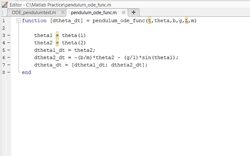
Code for function used in this program:

function [dtheta_dt] = pendulum_ode_func(t,theta,b,g,L,m)

    theta1 = theta(1)
    theta2 = theta(2)
    dtheta1_dt = theta2;
    dtheta2_dt = -(b/m)*theta2 - (g/1)*sin(theta1);
    dtheta_dt = [dtheta1_dt; dtheta2_dt];
end

5.OBSERVATION:

Output of Editor:

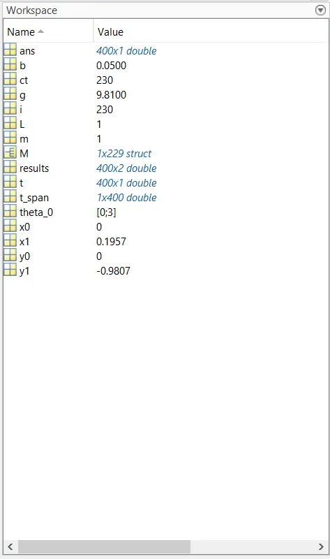
Output of Workspace:

Output of Function used in program:

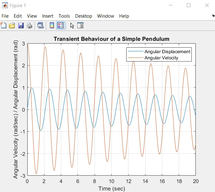
Output of graph:

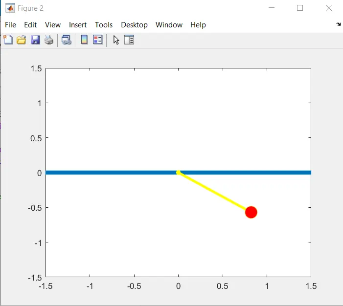
Video animation of Simple Pendulum

6.CONCLUSION:

• The graph of angular displacement and angular velocity plotted for the pendulum is sinusoidal in nature. The amplitude of motion reduces gradually as the motion is damped.