Assignment 4-RADIOSS Material Laws Challenge

Assignment 4

Aim

To compare and analyze the rupture plate simulation using different material properties

Procedure

• Import the failurejohnson_000.rad file to hypermesh

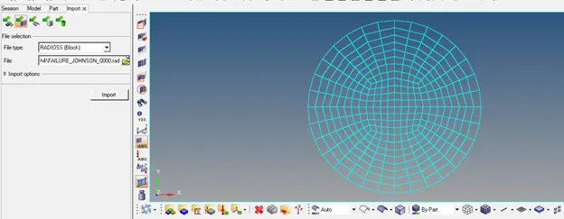
Figure 1

• After this, export the file to a new folder

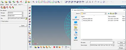
Figure 2

• An alternative is to simply name the file appropriately with a _0001.rad end so that radioss solver will identify it properly.
• The first case is the default simulation so simply go to analyse->radioss and run the analysis in the folder.

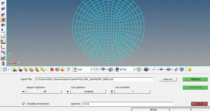
Figure3

• Note the input file should direct to a new folder as otherwise the files can get mixed up
• The various cases are shown in Table 1

Case 1	Run the default setup
Case 2	Make modifications to lfail_sh=1, Dadv=1 and lxfem =2 to the fail Johnson card. Refer Figure 4
Case 3	Delete the /fail/johnson card and run the simulation
Case4	Delete the value of EPS_p_max in the material aluminium card. Refer Figure 5
Case 5	Change the card image to law1 elastic with the same values of density, E and nu. Refer Figure 6
Case 6	Change the card image to law 36 with appropriate values
Case 7	Run law27_000.rad with the recommended property values

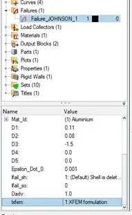
Figure 4

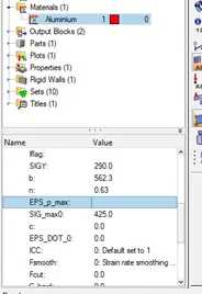
Figure 5

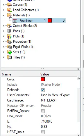
Figure 6

• In case 6, we make several changes to the material card.
• Firstly, we change it to law 36 Plastic Tabulated material and add the appropriate values.

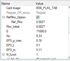
Figure 7

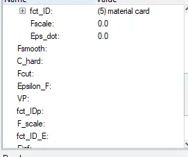
Figure 8

• For the function id, it is necessary to create a curve according to the values given in figure 9.

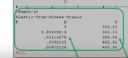
Figure 9

• Go to curves, and create a new curve.

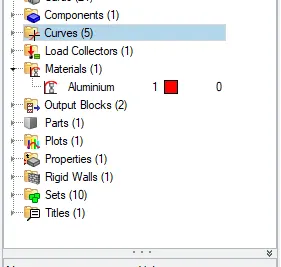
Figure 10

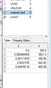
Figure 11

• Before we compare the graphs of the various cases, let us view the animations against each other with von mises contour enabled.

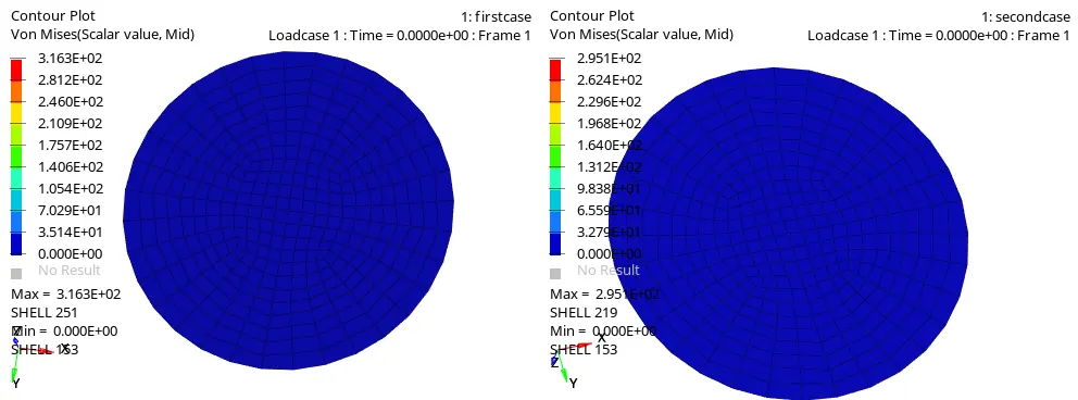
Figure 12

• At around t=4 or frame9, it can be easily observed that in case 2 the crack propagation is better defined and the stresses are more clear
• This can be attributed to the fact that in case 2, in the failure card, we set lfail_s=1, lx_fem=1 and dadv=1 which capture the animation more accurately.
• lfail Determines the Shell Element Failure Method
• lx_Fem determines whether failed elements crack or get deleted
• dadv determines how many pieces an element can break into before deletion

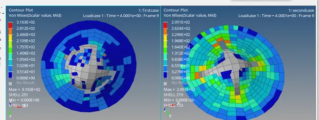
Figure 13

• In case3 the failure johnson card has been deleted.
• On comparing it with case 2, it can be observed that the failure of the component is more realistic in case 2 than in case 3 where the region fails uniformly.

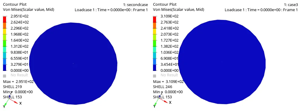
Figure 14

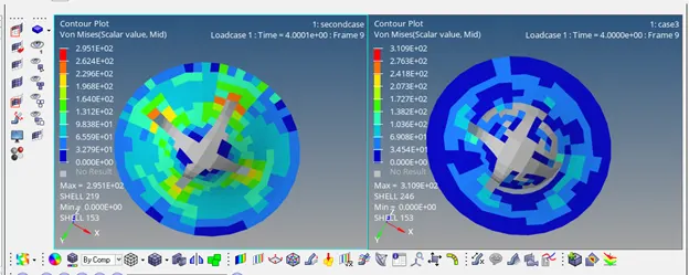
Figure 15

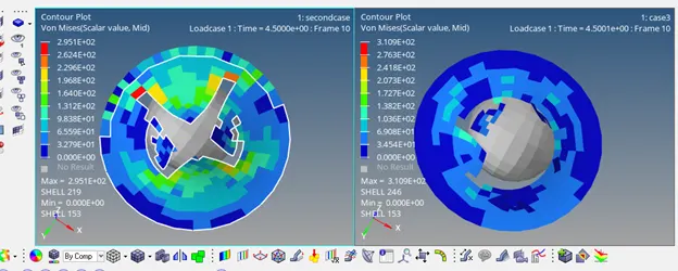
Figure 16

• In case 4, the value of Eps_max is deleted, this defaults to a very high value so failure is not observed in this animation

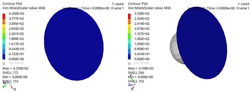
Figure 17

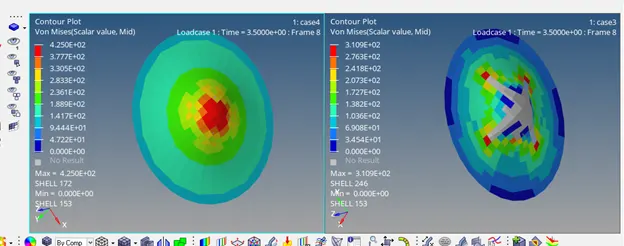
Figure 18

• In case 5, the Material card is changed to elastic.
• It can be observed that the stress distribution and deformation is more proper in case 5 over case 4
• The maximum stress experienced in case 5 is significantly more compared to that in case 4.

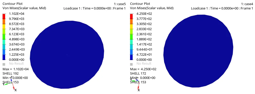
Figure 19

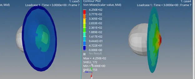
Figure 20

• In Case 6, the material card is changed to law36 Elasto Plastic.
• On comparing with Case 5 which had an elastic material card, we can clearly observe the difference as the component fails more explosively in case 6 which is usually what is observed with brittle materials

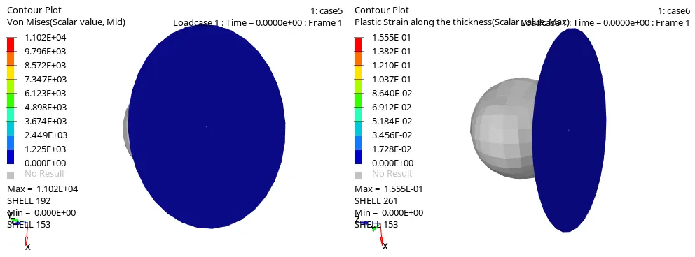
Figure 21

• In case 7, the material card is changed to Plastic Brittle.
• The difference can clearly be observed as there is plastic deformation in case 7
• After some plastic deformation, the region fails similar to brittle materials.

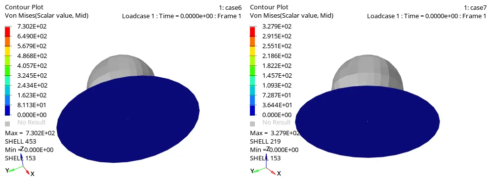
Figure 22

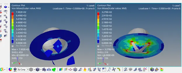
Figure 23

• Now, let us look at the graphs of each simulation.
• Case 1:In this case we are running the default simulation with the failure johnson card and having lx_fem lfail and dadv as
• The internal energy linearly increases up to 4ms after which it becomes constant

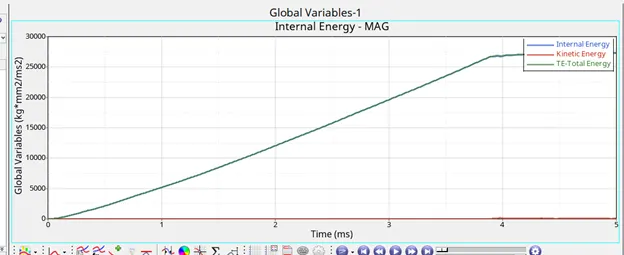
Figure 24

• This can be attributed to the fact that after 4ms failure occurs which result in element deletion.
• The spikes in kinetic energy further confirm this as element deletion allows the ball to move freely and resulting in element vibration around the region

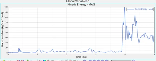
Figure 25

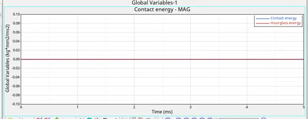
Figure 26

Simulation 2

• In this case, we modify the failure johnson card and set lfail_sh=1,dadv=2 and lx_fem=1.
• These modifications change the way failed elements react and thus enable us to properly visualize crack propagation
• This case is the most realistic scenario if the material used is aluminium.
• After around 4ms.the elements get deleted resulting in constant internal energy.

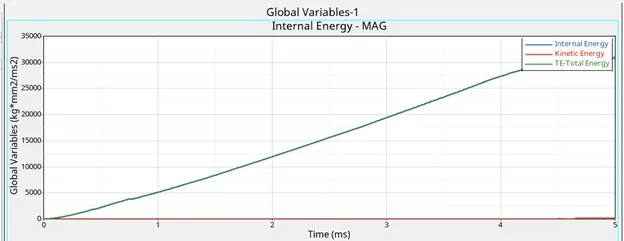
Figure 27

• The kinetic energy has a large spike after 4ms.suggesting element deletion and vibration in the region.

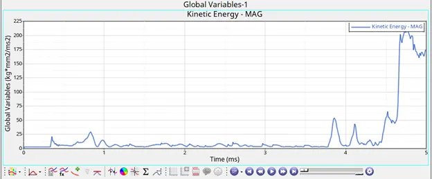
Figure 28

In case 3, the failure johnson card is deleted after which the simulation is run.

• Esp_max determines element failure, that is if the value of strain across any integration point crosses 15.1% of plastic strain they get deleted
• There is a linear increase in energy until a bulk of the elements get deleted

Figure 29

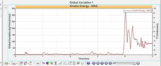
Figure 30

• In Case4, the Esp_Max value has been deleted.
• In this case, radioss assigns it an extremely high default value
• The material behaves like a pseudoelastic material since there are no failed elements to delete
• The kinetic energy, in this case, is negligible in comparison to the internal energy

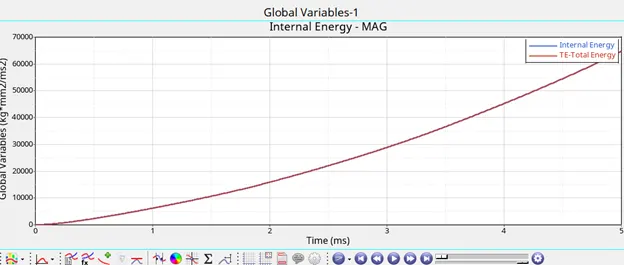
Figure 31

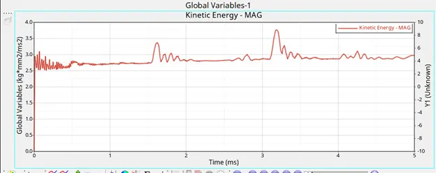
Figure 32

• In case 5, the material is law1 elastic with defines the basic properties of elastic materials
• It considers only the elastic phase of the materials, there is no plasticity, resulting in Linear Deformation. This purely elastic property assigned also results in no element failure.
• The kinetic energy gradually increases as the plate is stretched
• The internal energy increases exponentially due to the elastic nature of the material
• The maximum stress experienced by the plate is significantly larger compared to previous cases due to the elastic nature of the material

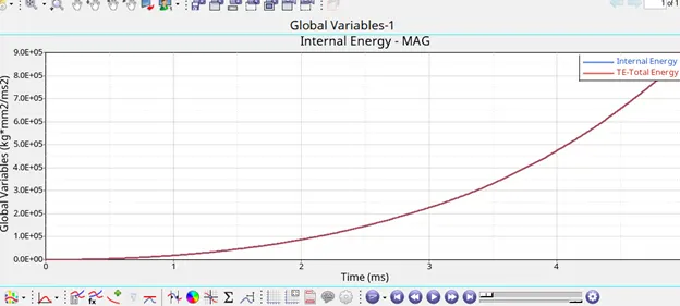
Figure 33

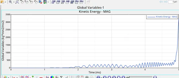
Figure 34

Case 6

• In this case, the material exhibits strongly brittle behaviour. There is no bending and it almost immediately breaks.
• There is no significant crack formation and the stress is not dissipated across the region. It is localized around the region of impact
• There is an almost linear relation between Internal energy and time until element failure after which it becomes constant.

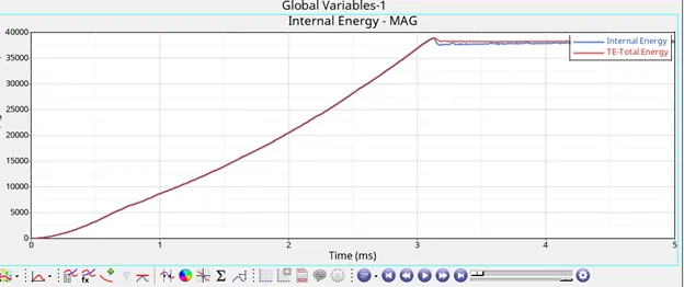
Figure 35

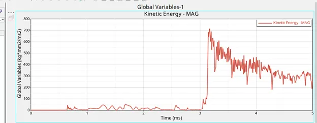
Figure 36

• In Case 7, we use Law 27 Plastic Brittle Material
• The sheet absorbs more force before failure in comparison to case 6
• The graph plateaus around the 4ms mark which coincides with element deletion

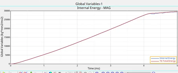
Figure 37

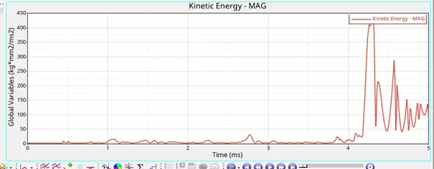
Figure 38

• Comparison between energy error%, mass error, element failure, no of cycles and solver time is given in table 2.

Case	Time Seconds	No of Cycles	Mass error	Energy Error %	Element Failure
1	442.11	49380	0	0.8	Deleted
2	651.67	49217	0	4.1	Elements crack before deformation
3	456	49408	0	0.8	Deleted
4	492.65	48737	0	3	No failure
5	388.43	47969	0	1.3	No failure
6	458.90	53143	0	-1.8	Deleted
7	408.75	49508	0	0.8%	Deleted

Learning Outcomes

• Commonly Used Material Cards in Radioss
• Failure Cards
• Comparing and analysing the animations using contour

Result

The various material cards commonly used in Radioss have been explored using a crash analysis of a plate.

Some common Material Cards include
Law1 Elastic

Law 2 Plastic

Law 27 Brittle
Law 36 Elastic-Plastic Behaviour modified with user-defined functions