Assignment 4-RADIOSS Material Laws Challenge

OBJECTIVE: To know about different material card in radioss and the difference in each material card.Also apply them in the given component and compare the result in tabulated format.

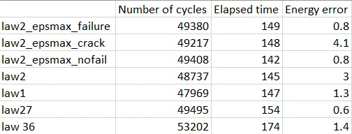
compare the total number of cycles, Energy error, mass error and simulation time in different cases and describe them briefly.

PROCEDURE:Import the given rad file into the radioss solver deck.

Go to file --> import --> solver deck. Select the RAD file and click import.

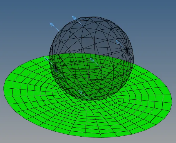
CASE 1:

Step I. In Radioss, Import FAILURE_JOHNSON_0000.rad starter file using Import Solver Deck menu.
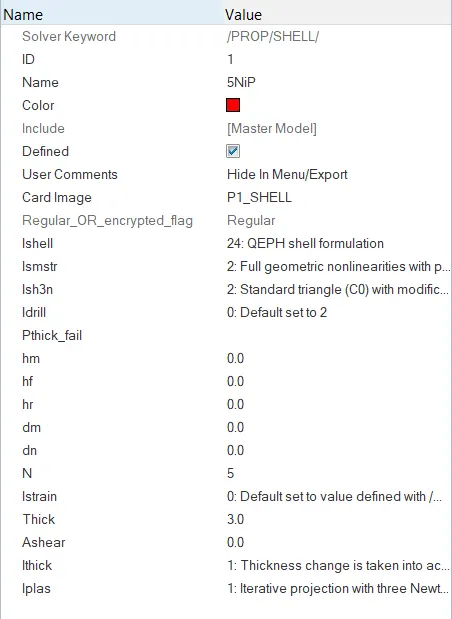
Step II. Go to properties and change the property values to the recommened values as shown below

STEP III: Then go to analysis tab and click radioss.

STEP IV: Now select the RAD file and run the simulation.

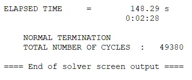
STEP V: Now open the output file and see the energy and mass error.

STEP VI. Then view the result in hyperview window for visualization.
STEP VII. Load .h3d file from specified path, play the animation and plot contour of Von Mises stress using Simple averaging method.
STEP VIII. Open HyperGraph 2D in a new window, load TO1 file and plot the energies required.

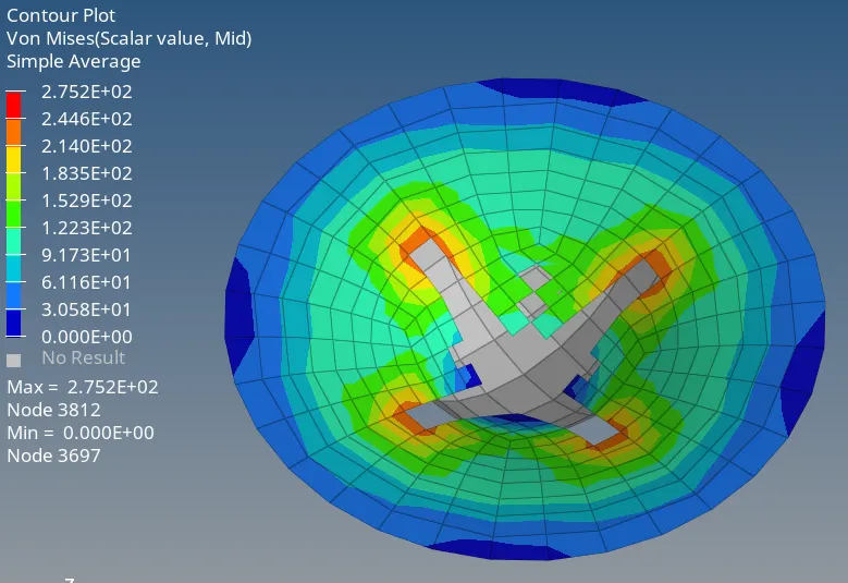
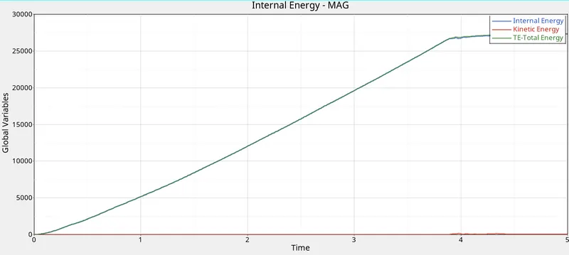
Law2 material is used in the above case which is johnson cook material model which represent the Isotropic Elasto-plastic material. In this model the maximum plastic strain is used for element failure and hence once the element reaches that particular value it deletes itself. In this model the total energy is almost same as the internal energy. In this the energy error is .8% which is acceptable.

CASE 2:

STEP I. In Radioss, Import FAILURE_JOHNSON_0000.rad starter file using Import Solver Deck menu.
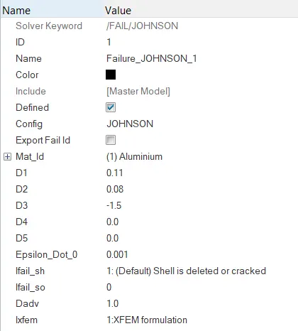
STEP II. Go to failure card and change the values to the given values as shown below

STEP III: Then go to analysis tab and click radioss.

STEP IV: Now select the RAD file and run the simulation.

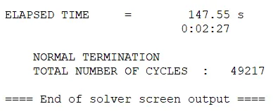
STEP V: Now open the output file and see the energy and mass error.

STEP VI. Then view the result in hyperview window for visualization.
STEP VII. Load .h3d file from specified path, play the animation and plot contour of Von Mises stress using Simple averaging method.
STEP VIII. Open HyperGraph 2D in a new window, load TO1 file and plot the energies required.

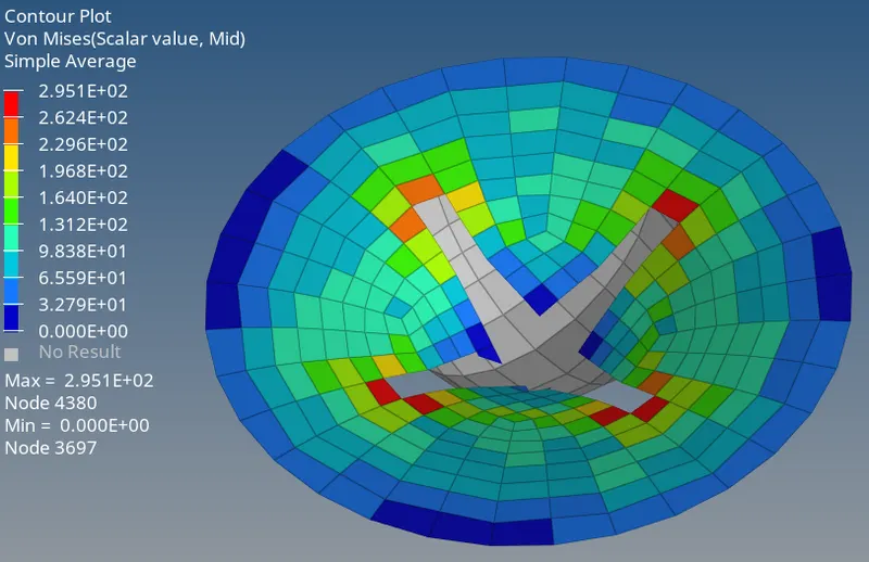
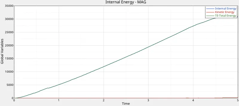
Law2 material is used in the above case which is johnson cook material model which represent the Isotropic Elasto-plastic material. In this model there are some changes that are made to the failure cards and as a result of that you can see the elements are being cracked and the internal energy is higher in this case than the previous case. In this case the energy error is 4.8% which is higher than the acceptable value that means there is some energy created in the system.

CASE 3:

STEP I. In Radioss, Import FAILURE_JOHNSON_0000.rad starter file using Import Solver Deck menu.
STEP II. Go to failure card and delete it.

STEP III: Then go to analysis tab and click radioss.

STEP IV: Now select the RAD file and run the simulation.

STEP V: Now open the output file and see the energy and mass error.

STEP VI. Then view the result in hyperview window for visualization.
STEP VII. Load .h3d file from specified path, play the animation and plot contour of Von Mises stress using Simple averaging method.
STEP VIII. Open HyperGraph 2D in a new window, load TO1 file and plot the energies required.

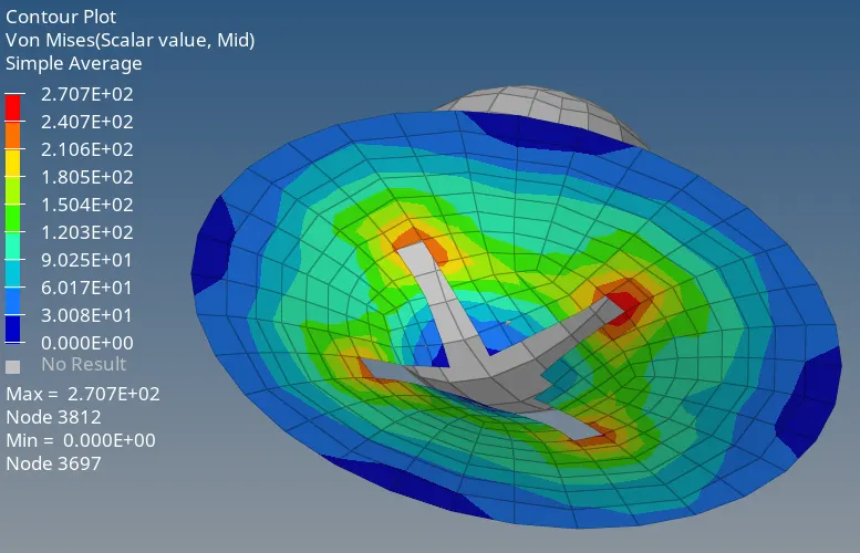
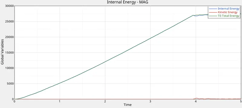
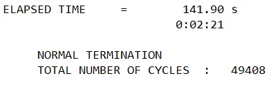
In this model the failure card is removed and the simulation is done. In This model the time taken is less and the energy values and stress are similar to the first case.

CASE 4:

STEP I. In Radioss, Import FAILURE_JOHNSON_0000.rad starter file using Import Solver Deck menu.
STEP II. Go to failure card and delete it. Then go to material property and delete the vlue of Eps_p_max value.

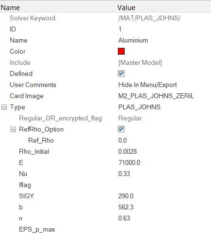
STEP III: Then go to analysis tab and click radioss.

STEP IV: Now select the RAD file and run the simulation.

STEP V: Now open the output file and see the energy and mass error.

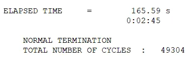
STEP VI. Then view the result in hyperview window for visualization.
STEP VII. Load .h3d file from specified path, play the animation and plot contour of Von Mises stress using Simple averaging method.
STEP VIII. Open HyperGraph 2D in a new window, load TO1 file and plot the energies required.

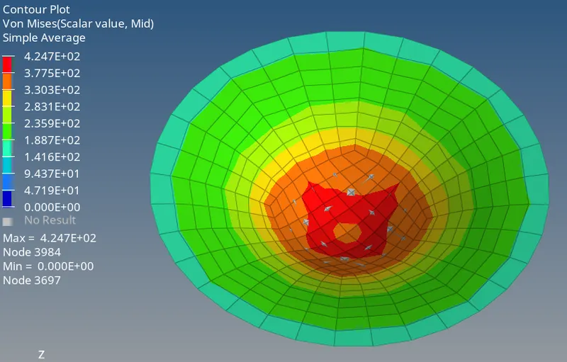
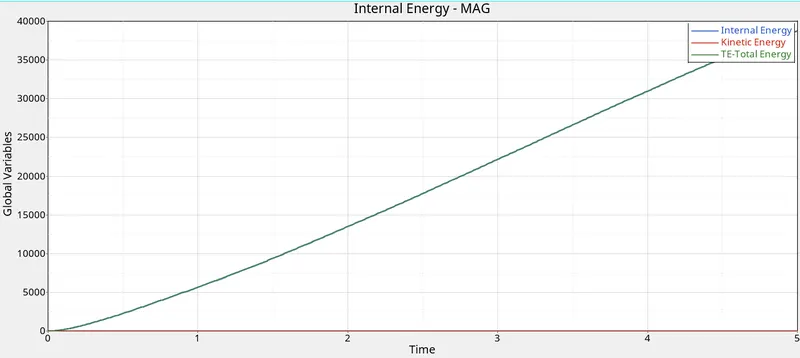
In this model the maximum plastic strain is removed hence the elements are not failed and thus all the elements are present. In this the value of stress is high when compared to other elements as there is no failing value for the elements.The value of energy is gradually increasing.

CASE 5:

STEP I. In Radioss, Import FAILURE_JOHNSON_0000.rad starter file using Import Solver Deck menu.
STEP II. Go to material card and change the material to law 1 elastic material.

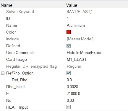
STEP III: Then go to analysis tab and click radioss.

STEP IV: Now select the RAD file and run the simulation.

STEP V: Now open the output file and see the energy and mass error.

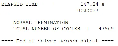
STEP VI. Then view the result in hyperview window for visualization.
STEP VII. Load .h3d file from specified path, play the animation and plot contour of Von Mises stress using Simple averaging method.
STEP VIII. Open HyperGraph 2D in a new window, load TO1 file and plot the energies required.

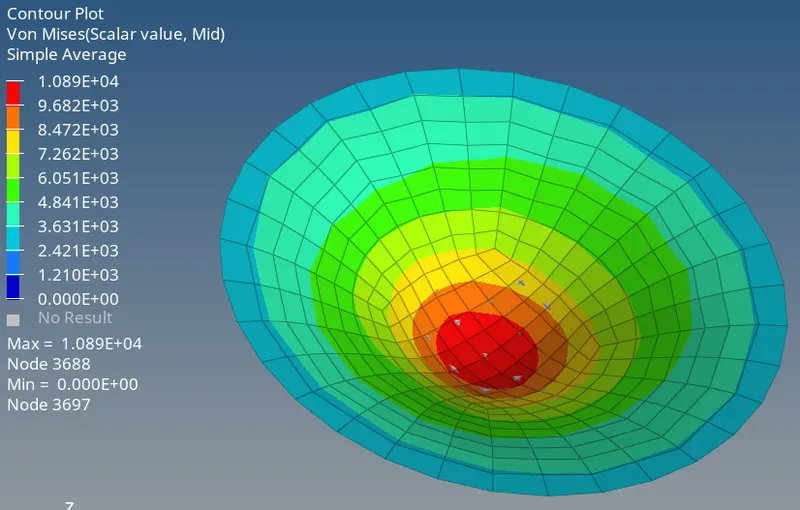
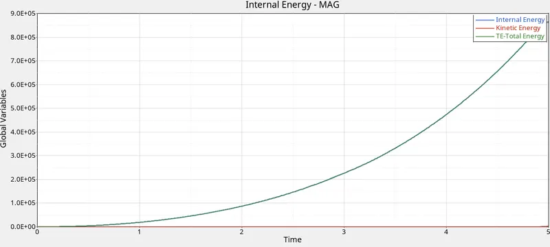
Law1 material is used in the above case which is elastic material model. In this model the stress value increases to a greater extent as it has linear property between stress and strain.The internal energy for elastic material is also very high.

CASE 6:

STEP I. In Radioss, Import FAILURE_JOHNSON_0000.rad starter file using Import Solver Deck menu.
STEP II. Go to property card and change the property to the recommended value.

STEP III: Then go to analysis tab and click radioss.

STEP IV: Now select the RAD file and run the simulation.

STEP V: Now open the output file and see the energy and mass error.

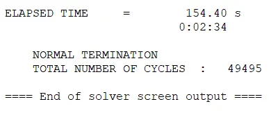
STEP VI. Then view the result in hyperview window for visualization.
STEP VII. Load .h3d file from specified path, play the animation and plot contour of Von Mises stress using Simple averaging method.
STEP VIII. Open HyperGraph 2D in a new window, load TO1 file and plot the energies required.

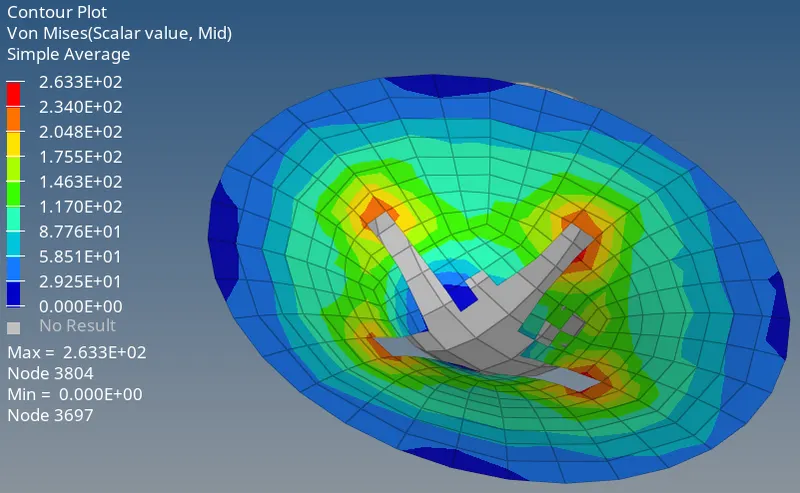
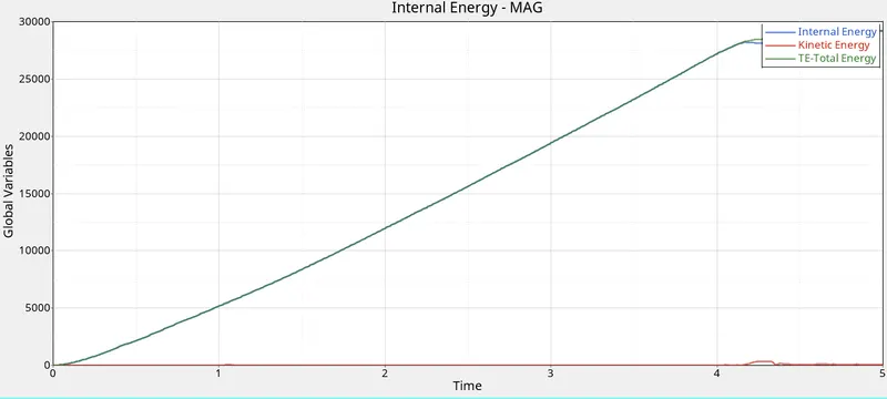
In this model, we used LAW27 which combines an isotropic elasto-plastic Johnson-Cook material model with an orthotropic brittle failure
model.Thus we can see the brittle failure in the simulation which creates some deviation in the energy graph.

CASE 7:

STEP I. In Radioss, Import FAILURE_JOHNSON_0000.rad starter file using Import Solver Deck menu.
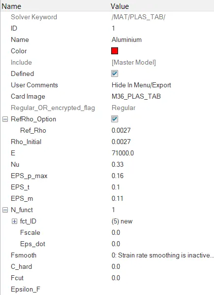
STEP II. Go to curve card and plot a new curve with the given values and then change the material property to law36.

STEP III: Then go to analysis tab and click radioss.

STEP IV: Now select the RAD file and run the simulation.

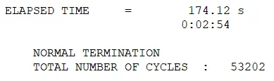
STEP V: Now open the output file and see the energy and mass error.

STEP VI. Then view the result in hyperview window for visualization.
STEP VII. Load .h3d file from specified path, play the animation and plot contour of Von Mises stress using Simple averaging method.
STEP VIII. Open HyperGraph 2D in a new window, load TO1 file and plot the energies required.

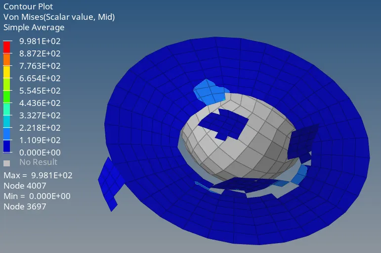
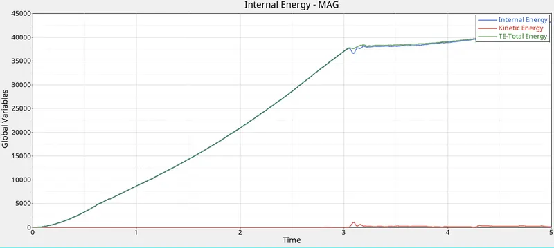
This model uses the law36 material which is a isotropic elasto-plastic material using user define function.In this model the stress values are higher when compared to other model.In this model the internal energy is also high.

A tabulation of the above results are made and is shown below