Assignment 4-RADIOSS Material Laws Challenge
Objective:
Perform the simulation as per the cases given below
Case 1
- Import the FAILURE_JOHNSON_0000.rad file and run the model as it is. Give the title name as Law2_epsmax_failure.
Case 2
- Import the case 1 rad file, named "Law2_epsmax_failure" and perform the simulation with failure plastic (EPS_p_max) and fail_Johnson card enabled.
- Changes to be made in /FAIL/JOHNSON card:
- ifail_sh = 1
- Dadv = 1
- Ixfem = 1
- Use the recommended values for the property card.
- Give the title name as Law2_epsmax_crack.
Case 3
- Import the case 2 rad file, named "Law2_epsmax_crack" and perform the simulation by removing the fail_Johnson failure card. Give the title name as Law2_epsmax_nofail.
Case 4
- Import the case 3 rad file, named "Law2_epsmax_nofail" and perform the simulation by removing both the plastic stain (EPS_p_max) and the fail_Jhonson failure card.
Case 5
- Import the case 4 rad file and perform the simulation by changing the material card to Law 1. Keep the same value for rho, E and nu values.
Case 6
- Import the case 1 rad file, named "Law2_epsmax_failure" and perform the simulation with the law 36 material card. Refer to the video titled "Materials 7 for further information.
Case 7
- Open the Law27_0000.rad file and perform the simulation with the law 27 material card. Use the recommended shell properties.
Procedure:
Case 1
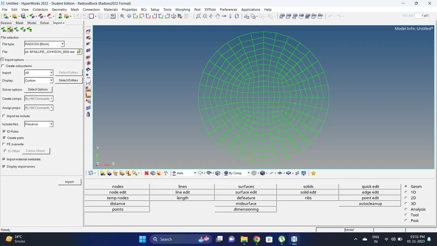
1. Open the Hypermesh in Radioss profile and import the FAILURE_JOHNSON_0000.rad file.
2. Run the simulation
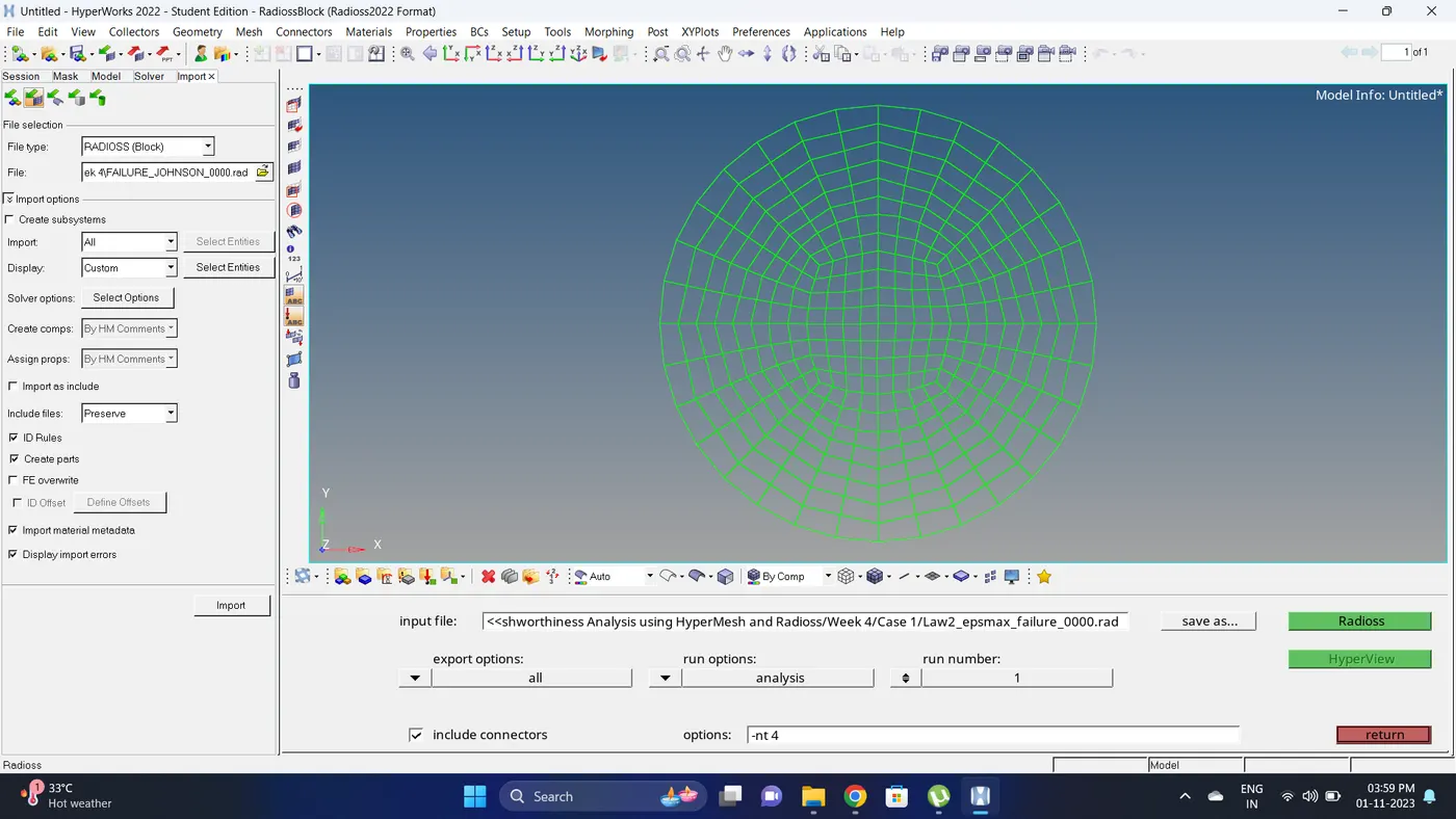
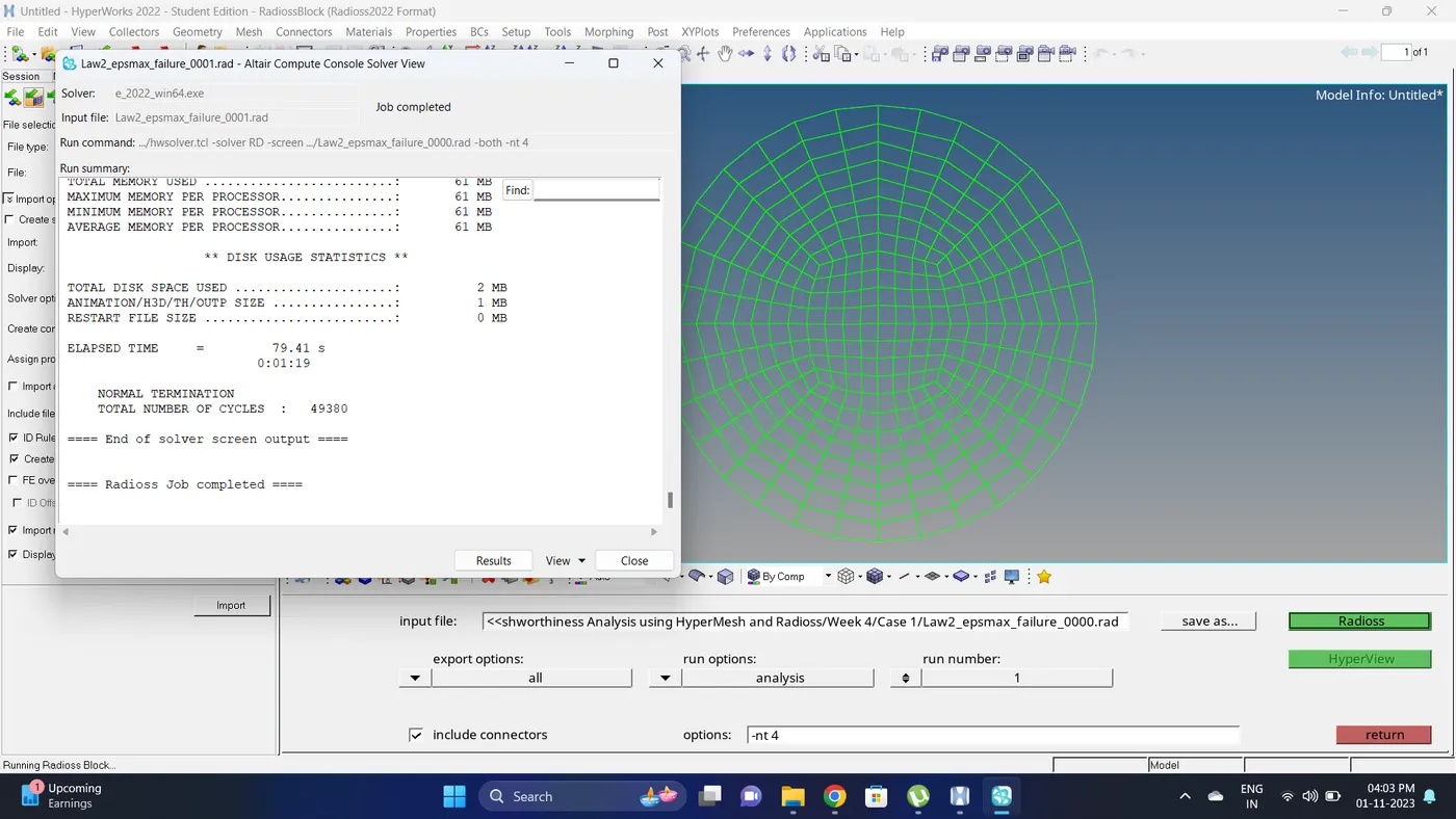
Go to Analysis - Radioss - click on save as, Rename the file to Law2_epsmax_failure and at the end type .rad - Ensure that export option is set to all and Include connectors is tick - Click Radioss to run the simulation.
Note: If the stimulation is not running it taking time then copy the given input 0000.rad and 0001.rad file to folder, Rename both the file to Law2_epsmax_failure, click on the 0000.rad file click save and overwrite it.
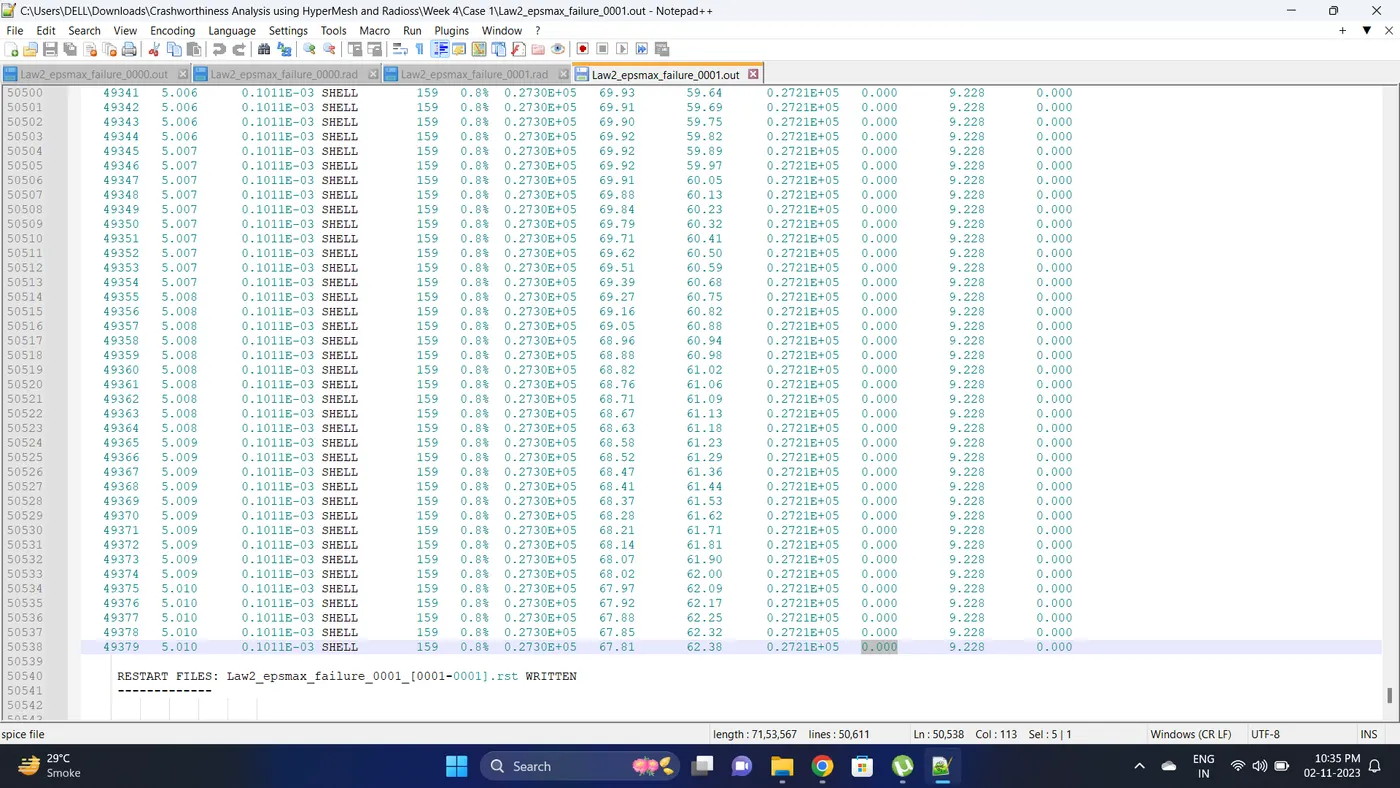
3. Open 0001.out file in notepad ++ and check the maximum total energy error and mass error.
The torelance for the energy error is -15 to +5 % and mass error is upto 2 %
Energy error is 0.8%
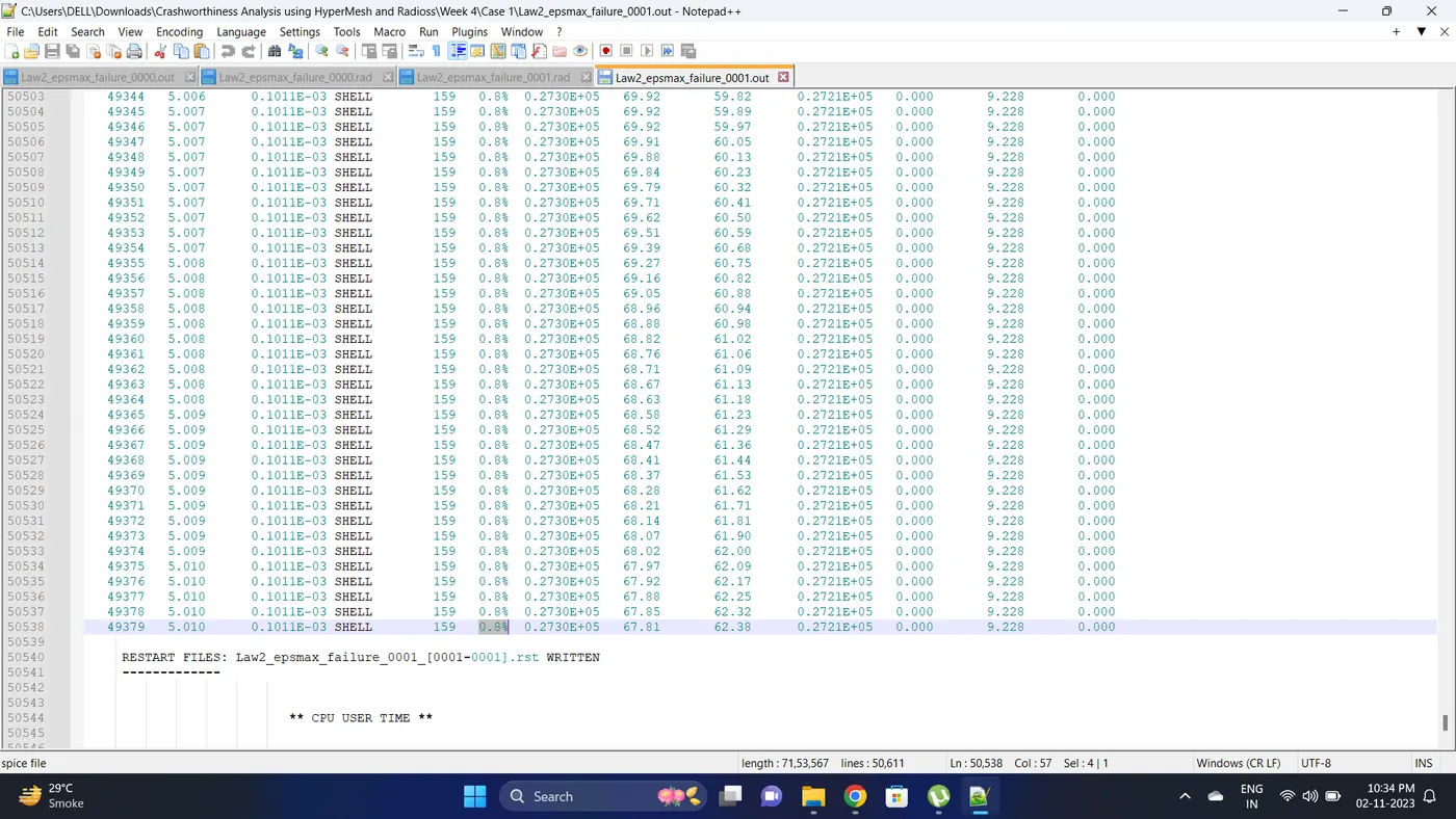
Mass error is 0 %
4. Open the Hyperwork in Hypergraph 2D view.
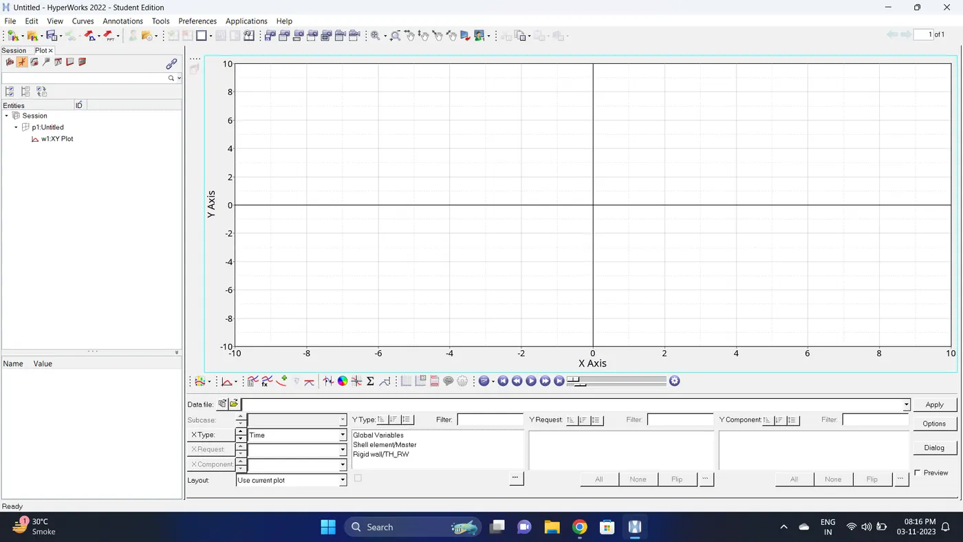
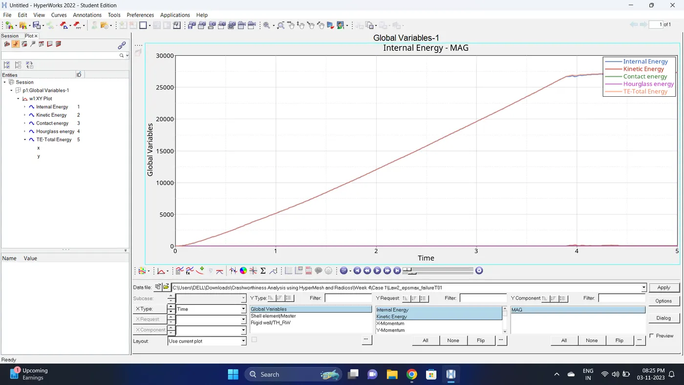
5. Open the T01 file from case_1 and select the Global Variable - Internal energy, Kinetic energy, Contact Energy, Hourglass Energy and Total Energy - Click apply to plot the graph.
6. Note down the minimum and maximum value of various Energy by right click on any energy - Single curve math - Min Note. similarly do for maximum
Note: after getting graph reading turn off that graph and do next reading.
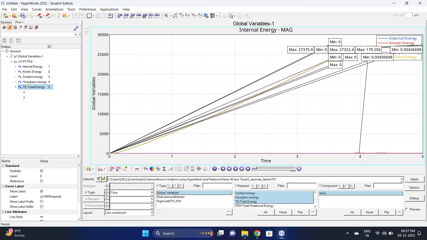
| Sr.no | Name | Minimum | Maximum |
| 1 | Internal Energy | 0 | 27322.4 |
| 2 | Kinetic Energy | 0.00436698 | 179.256 |
| 3 | Contact Energy | 0 | 0 |
| 4 | Hourglass Energy | 0 | 0 |
| 5 | Total Energy | 0.00436698 | 27375.9 |
7. Open the Hyperwork in Hyperview view.
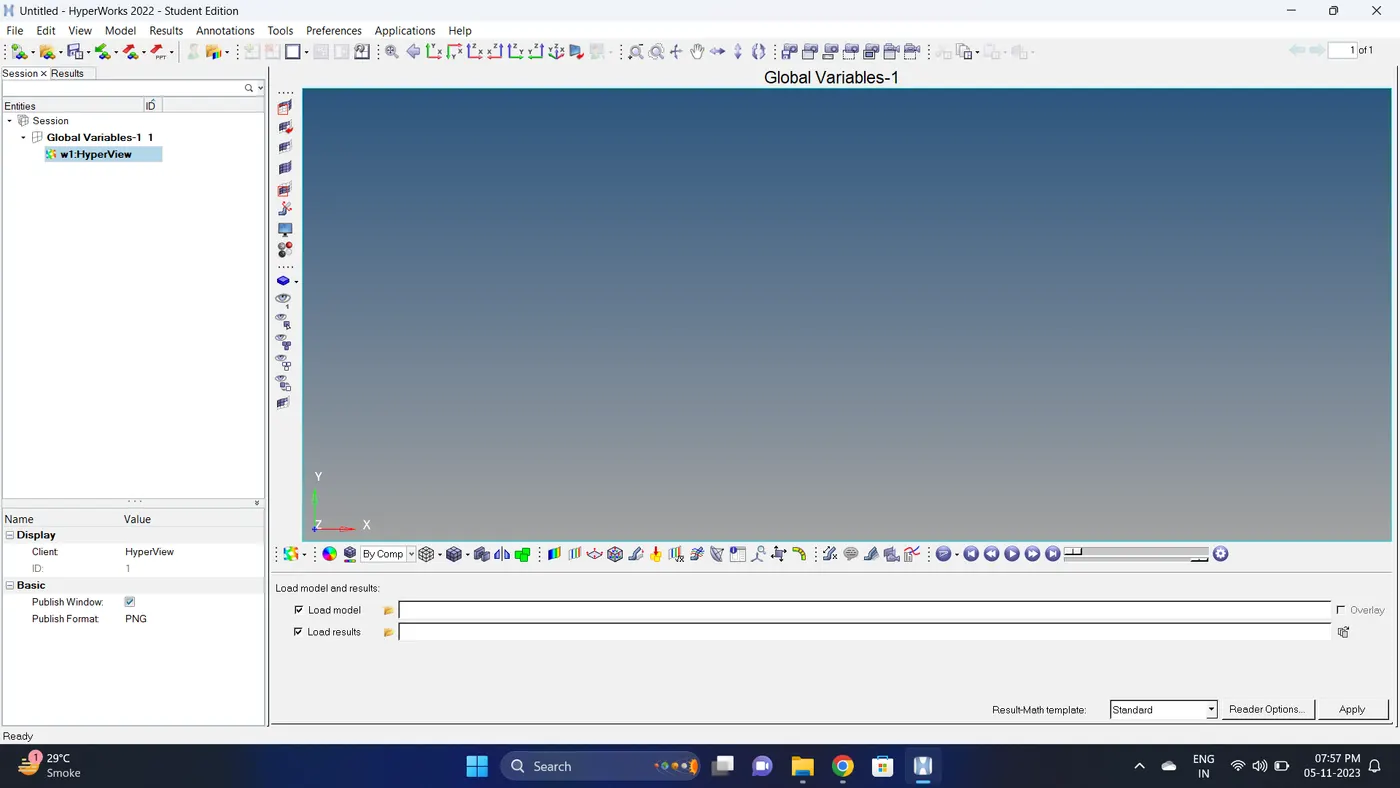
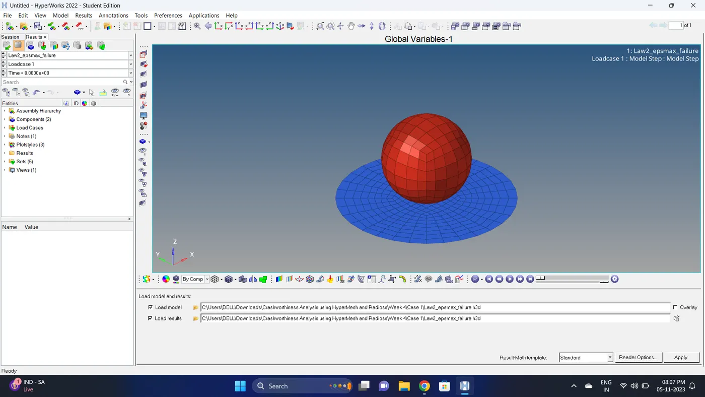
8. Import the .h3d file.
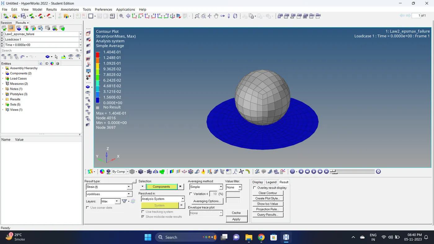
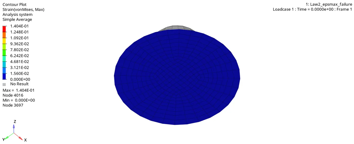
9. Go to the contour - change result type to strain (t), averaging method to simple, click on apply and play the animation.
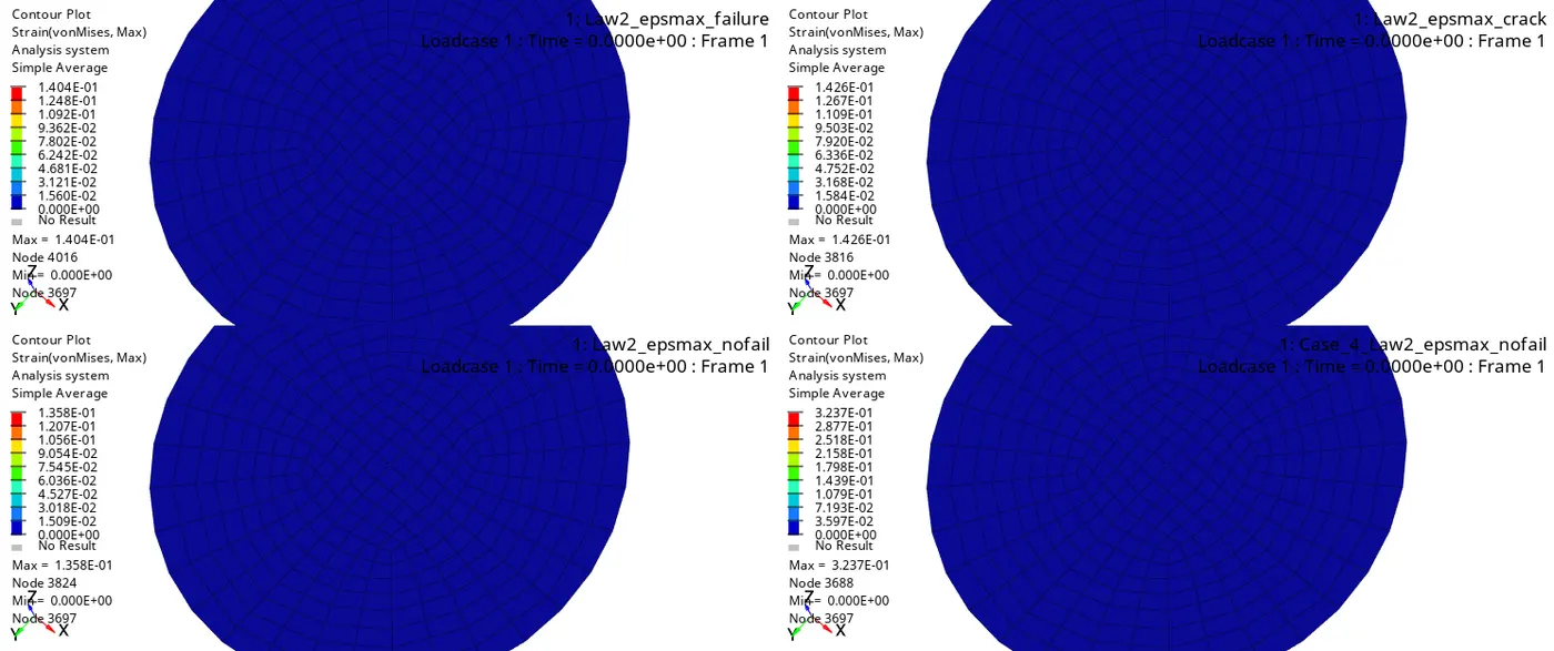
Maximum strain = 0.1404 and Minimum stain is 0
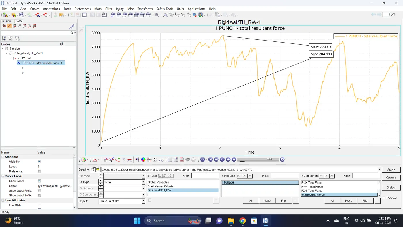
10. Plot the rigid wall forces.
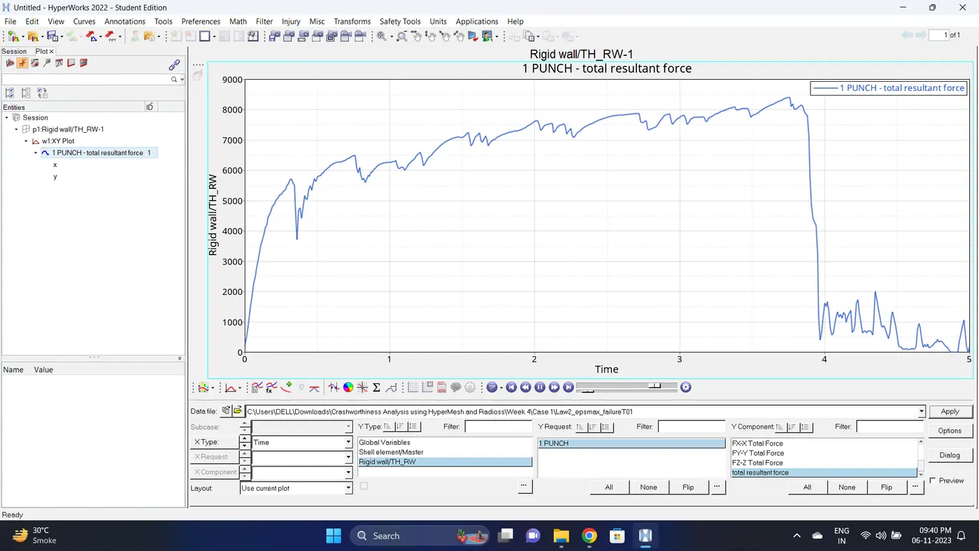
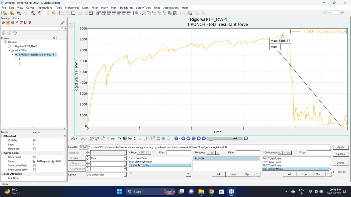
Case 2
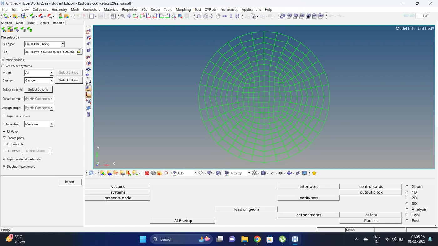
1. Import the case 1 rad file, named “Law2_epsmax_failure”.
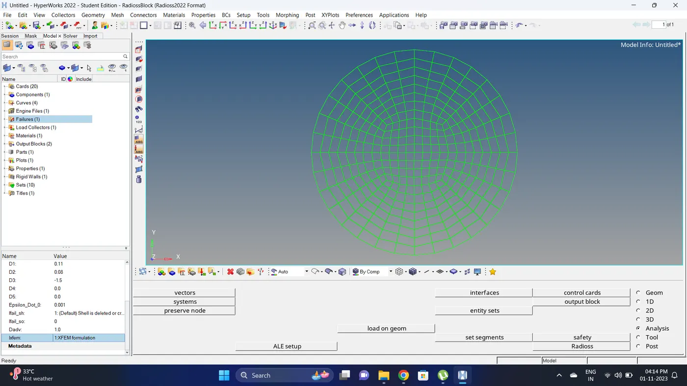
2. Go to the model browser - Failures - change the value of ifail_sh= 1, Dadv= 1 and Ixfem= 1.
3. Run the simulation
Go to Analysis - Radioss - click on save as, Rename the file to Law2_epsmax_crack and at the end type .rad - Ensure that export option is set to all and Include connectors is tick - Click Radioss to run the simulation.
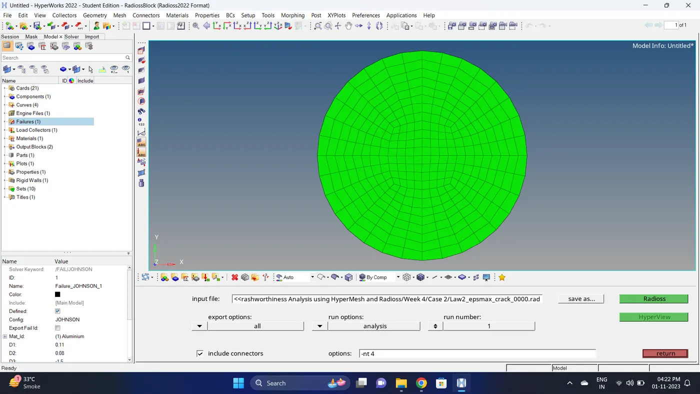
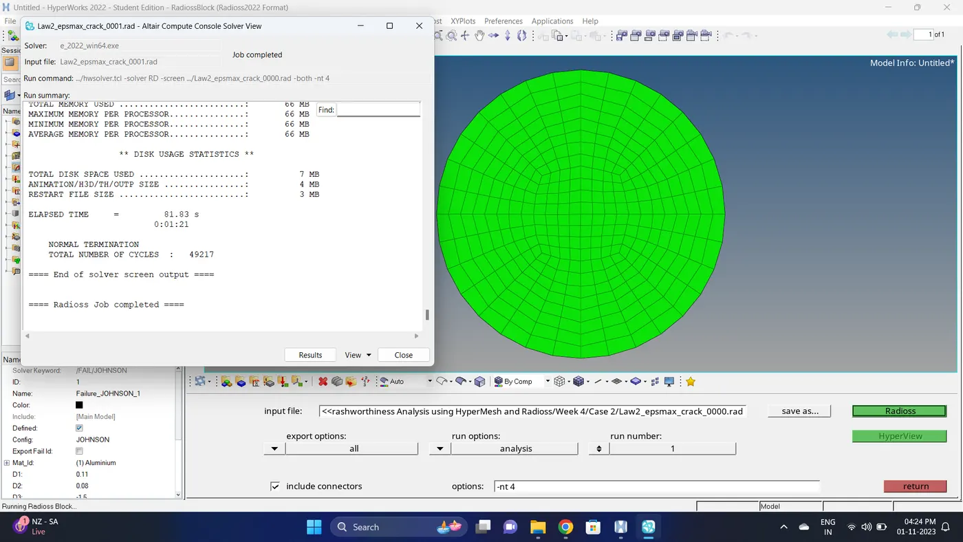
4. Open 0001.out file in notepad ++ and check the maximum total energy error and mass error.
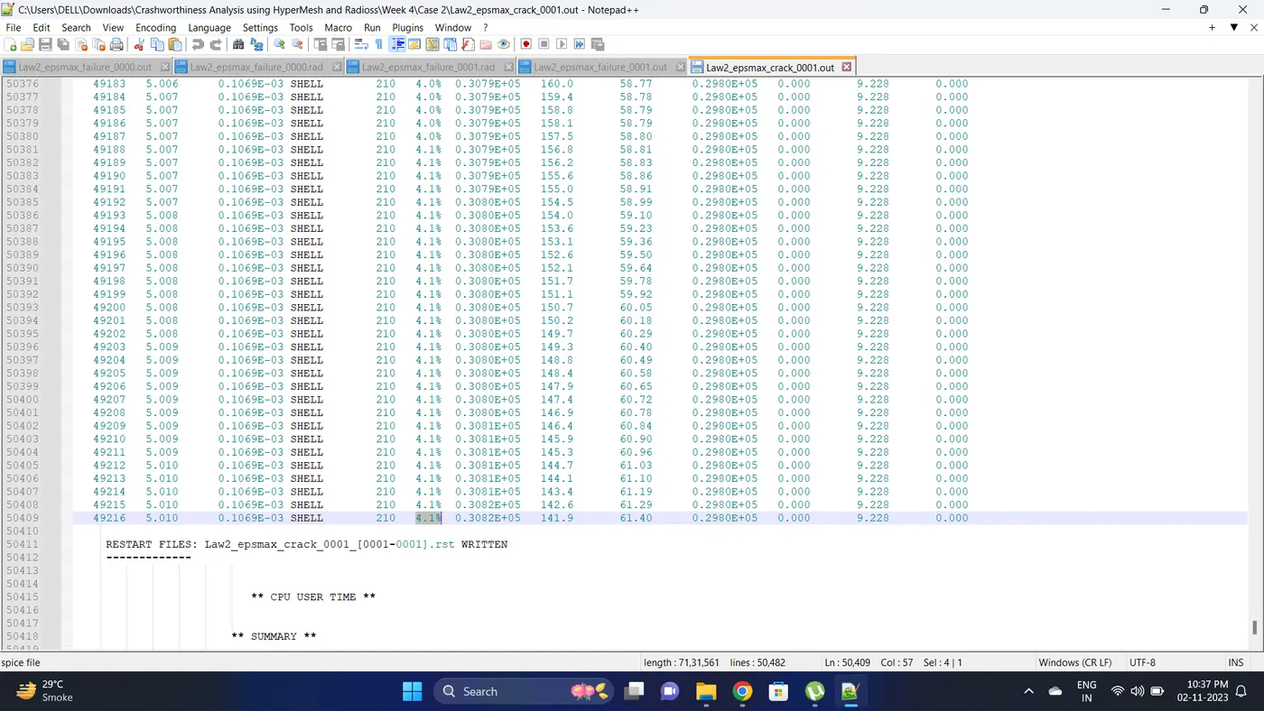
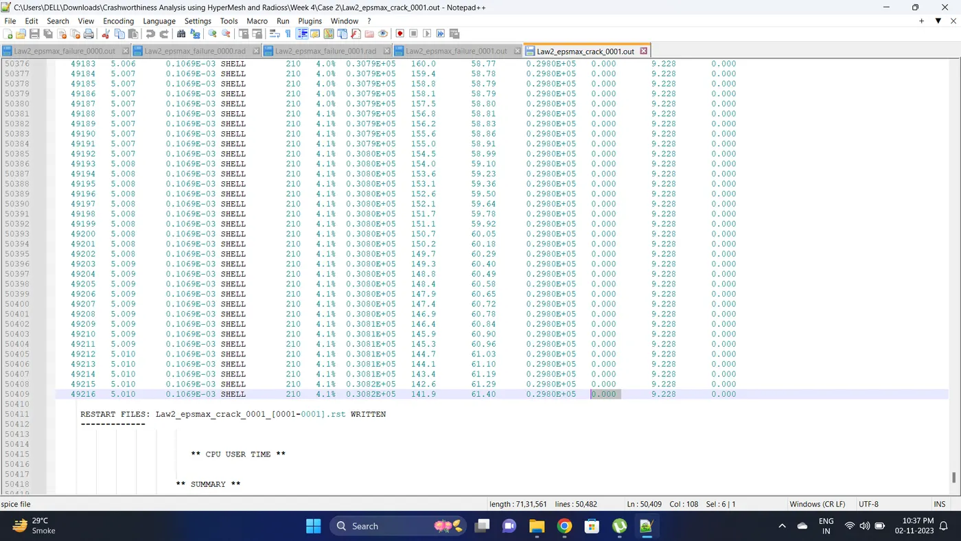
The torelance for the energy error is -15 to +5 % and mass error is upto 2 %
Energy error is 4.1 %
Mass error is 0 %
5. Open the Hyperwork in Hypergraph 2D view.
6. Open the T01 file from case_2 and select the Global Variable - Internal energy, Kinetic energy, Contact Energy, Hourglass Energy and Total Energy - Click apply to plot the graph.
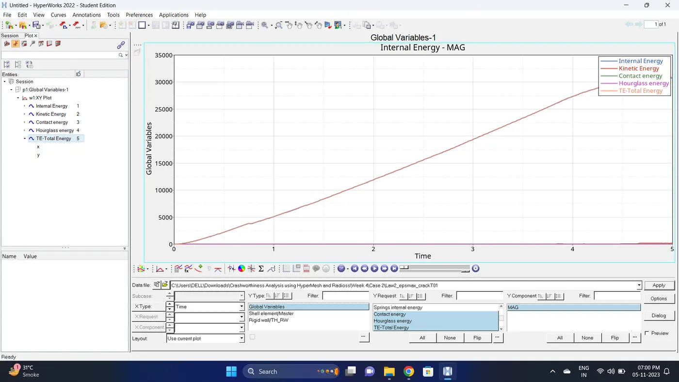
7. Note down the minimum and maximum value of various Energy by right click on any energy - Single curve math - Min Note. similarly do for maximum
Note: after getting graph reading turn off that graph and do next reading.
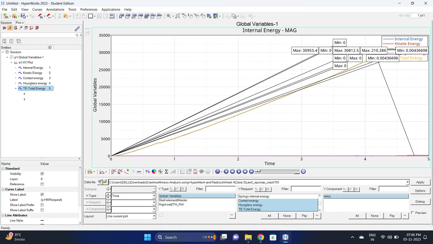
| Sr.no | Name | Minimum | Maximum |
| 1 | Internal Energy | 0 | 30812.5 |
| 2 | Kinetic Energy | 0.00436698 | 210.286 |
| 3 | Contact Energy | 0 | 0 |
| 4 | Hourglass Energy | 0 | 0 |
| 5 | Total Energy | 0.00436698 | 30953.4 |
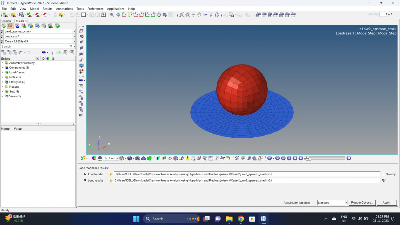
8. Open the Hyperwork in Hyperview view.
9. Import the .h3d file.
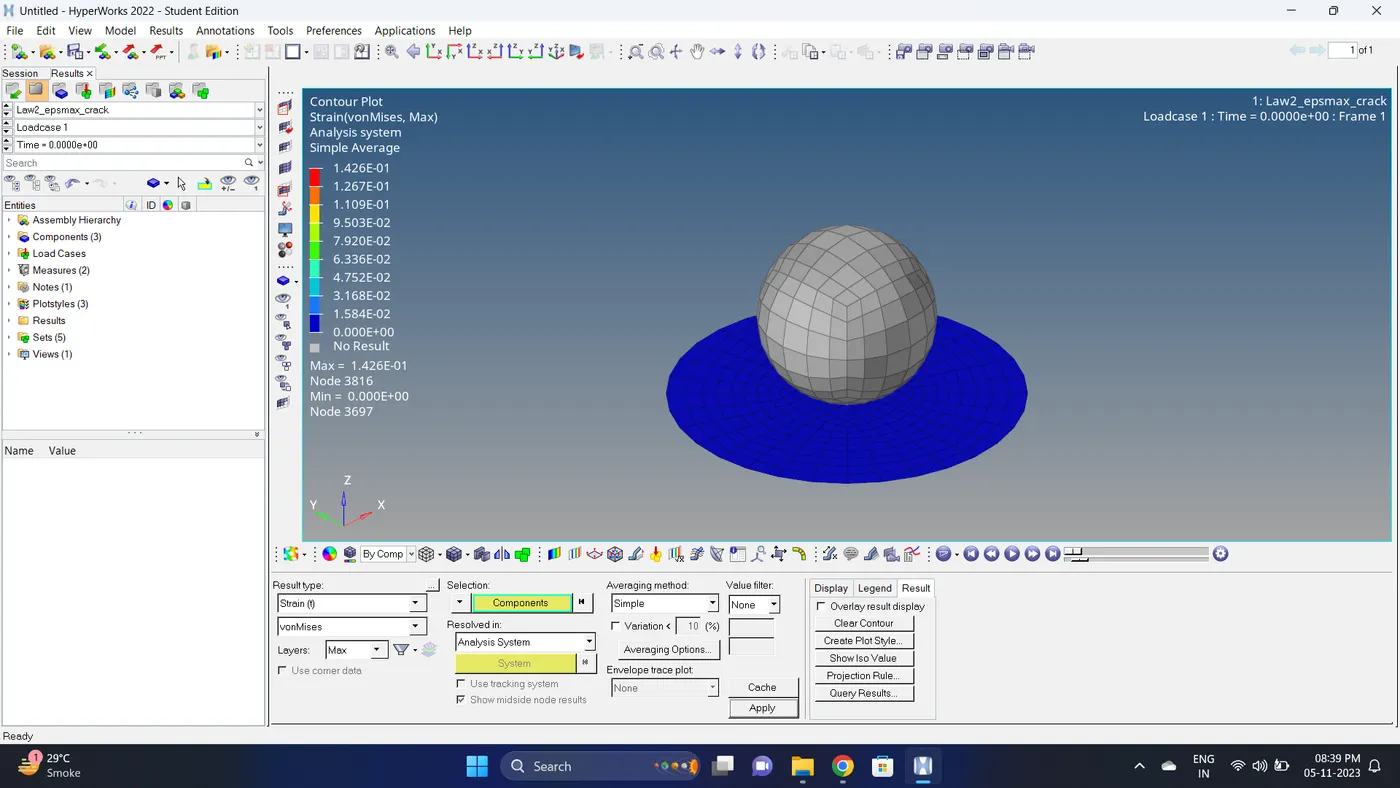
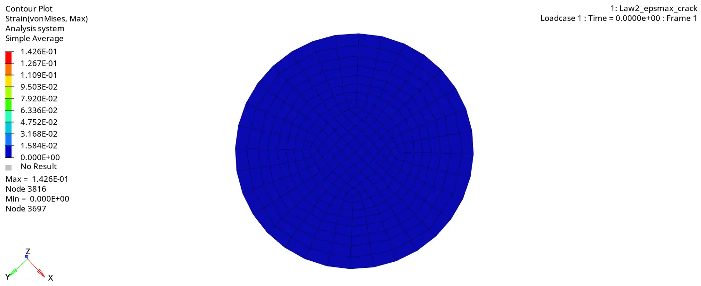
10. Go to the contour - change result type to strain (t), averaging method to simple, click on apply and play the animation.
Maximum strain = 0.1426 and Minimum stain is 0
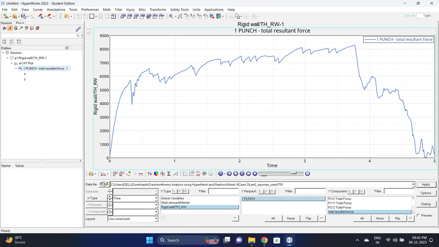
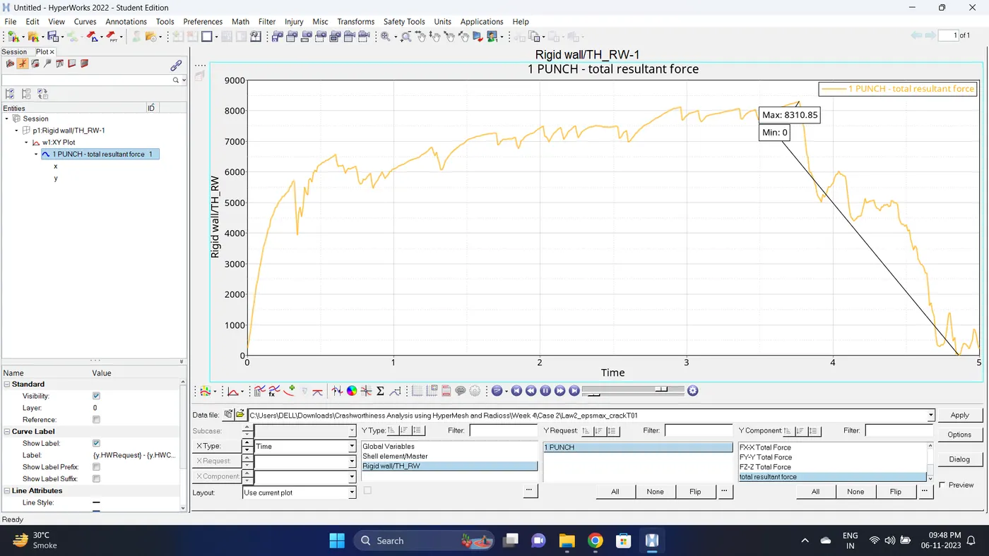
11. Plot the rigid wall forces.
Case 3
1. Import the case 2 rad file, named “Law2_epsmax_crack”
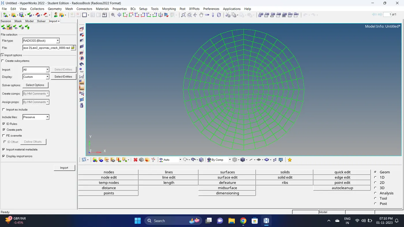
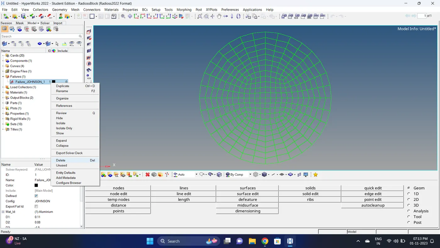
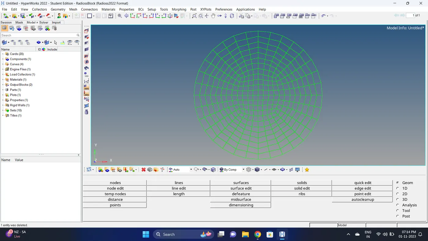
2. Delete the Failure_Johnson card.
3. Run the simulation
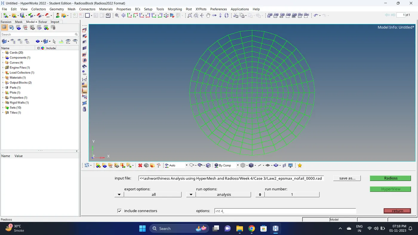
Go to Analysis - Radioss - click on save as, Rename the file to Law2_epsmax_nofail and at the end type .rad - Ensure that export option is set to all and Include connectors is tick - Click Radioss to run the simulation.
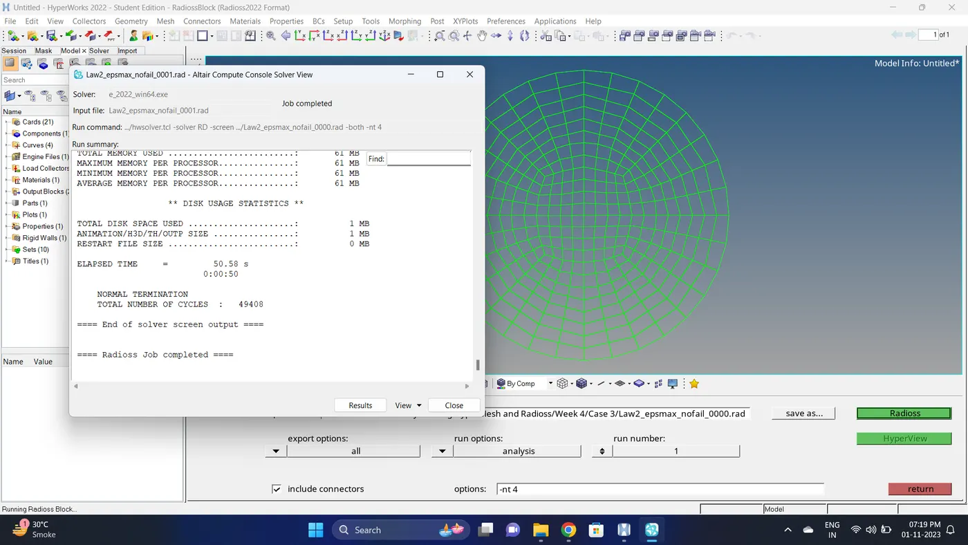
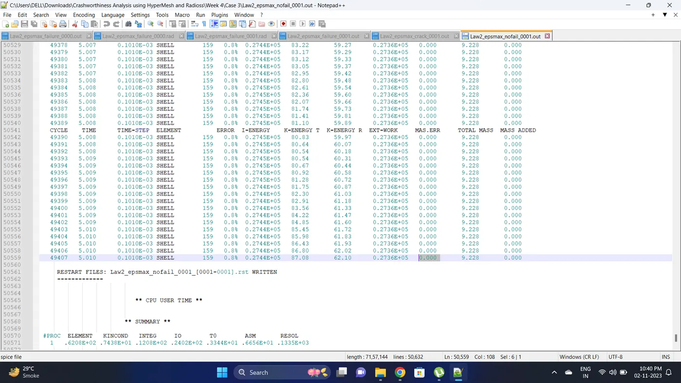
4. Open 0001.out file in notepad ++ and check the maximum total energy error and mass error.
The torelance for the energy error is -15 to +5 % and mass error is upto 2 %
Energy error is 0.8 %
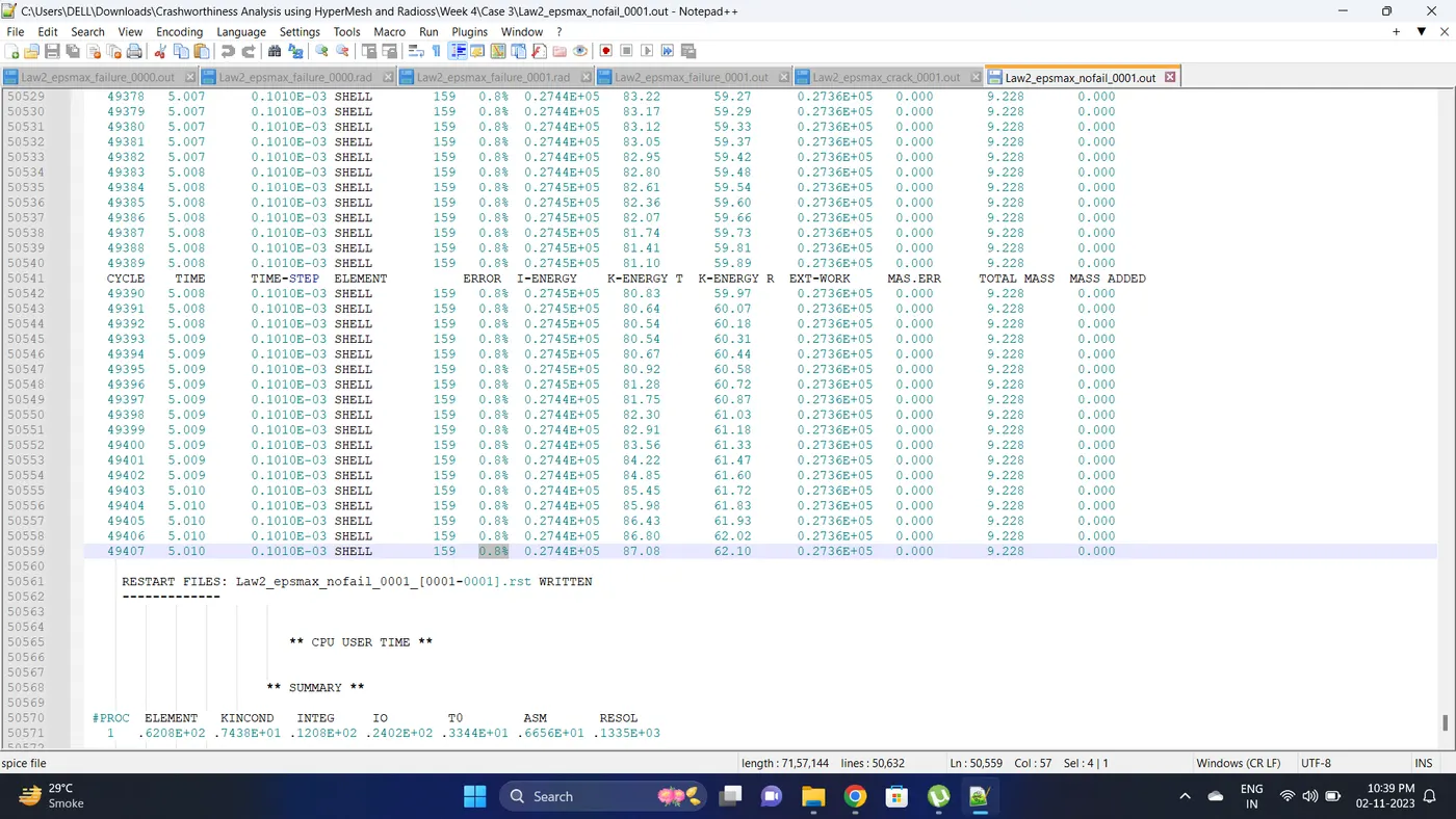
Mass error is 0 %
5. Open the Hyperwork in Hypergraph 2D view.
6. Open the T01 file from case_3 and select the Global Variable - Internal energy, Kinetic energy, Contact Energy, Hourglass Energy and Total Energy - Click apply to plot the graph.
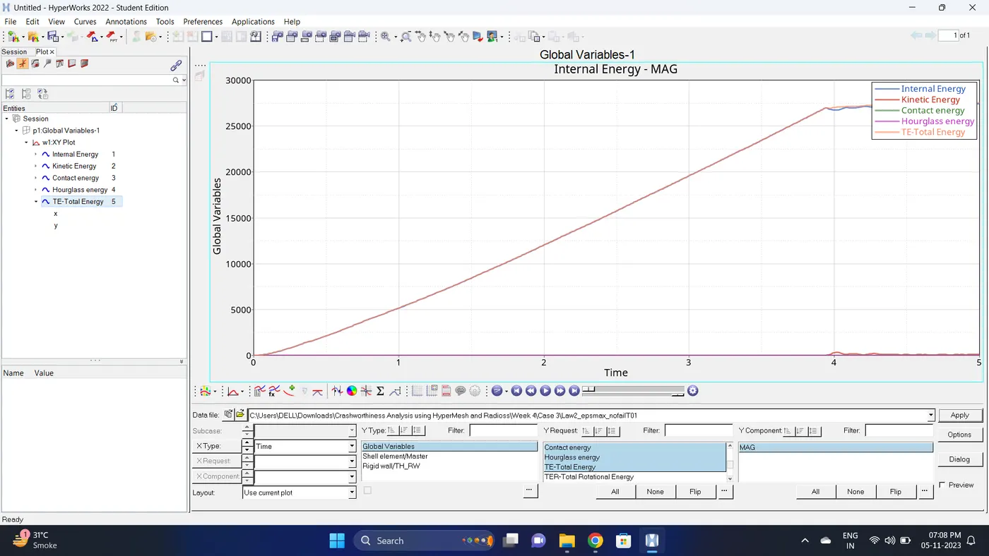
7. Note down the minimum and maximum value of various Energy by right click on any energy - Single curve math - Min Note. similarly do for maximum
Note: after getting graph reading turn off that graph and do next reading.
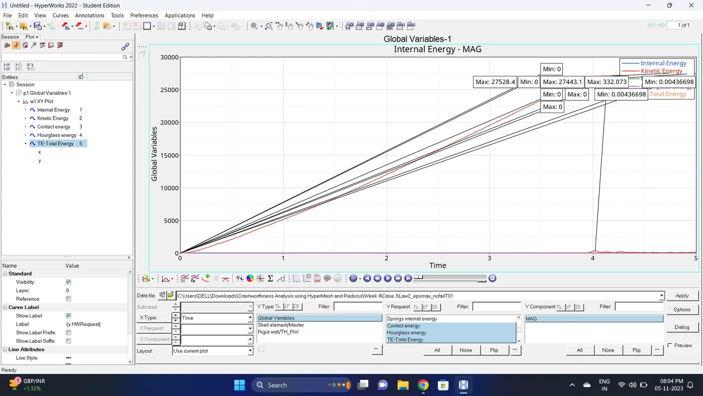
| Sr.no | Name | Minimum | Maximum |
| 1 | Internal Energy | 0 | 27443.1 |
| 2 | Kinetic Energy | 0.00436698 | 332.073 |
| 3 | Contact Energy | 0 | 0 |
| 4 | Hourglass Energy | 0 | 0 |
| 5 | Total Energy | 0.00436698 | 27528.4 |
8. Open the Hyperwork in Hyperview view.
9. Import the .h3d file.
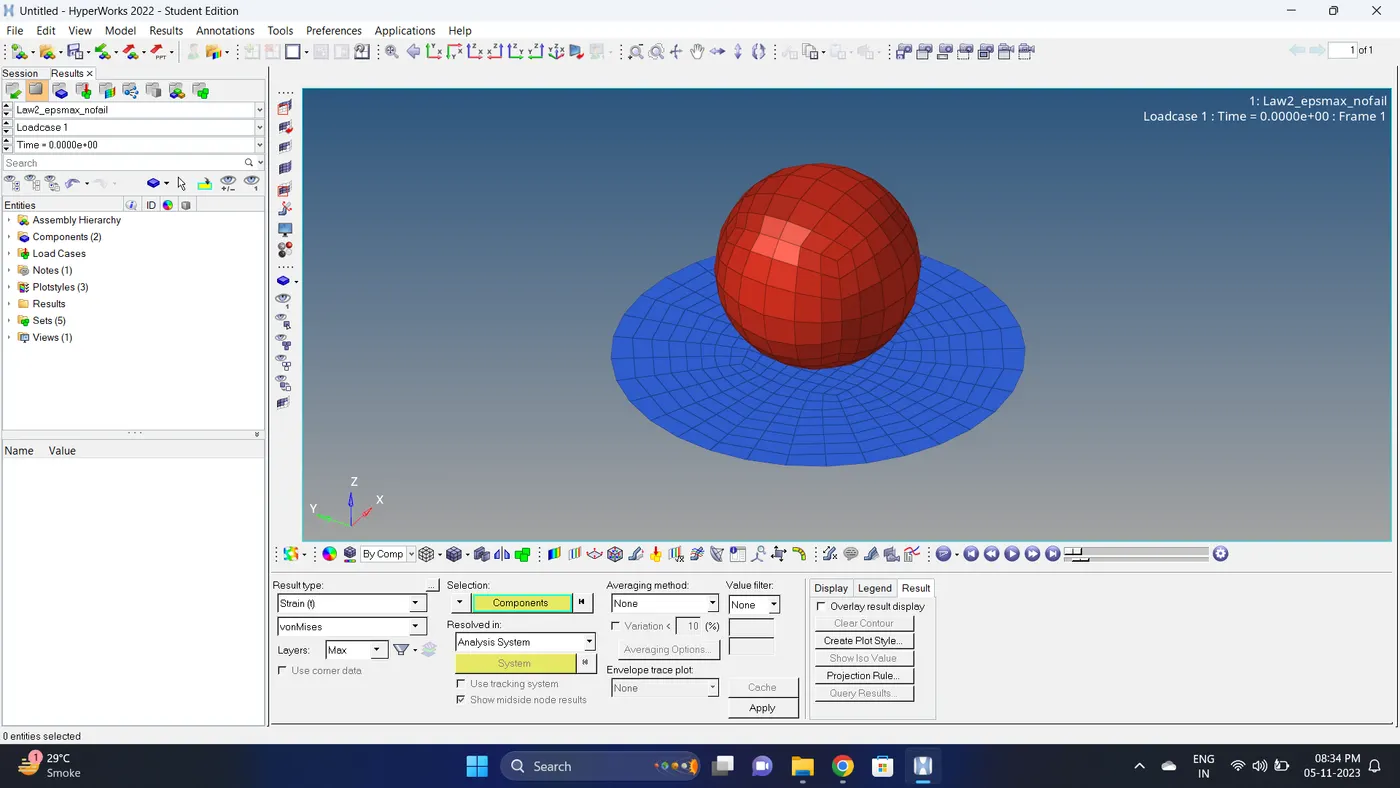
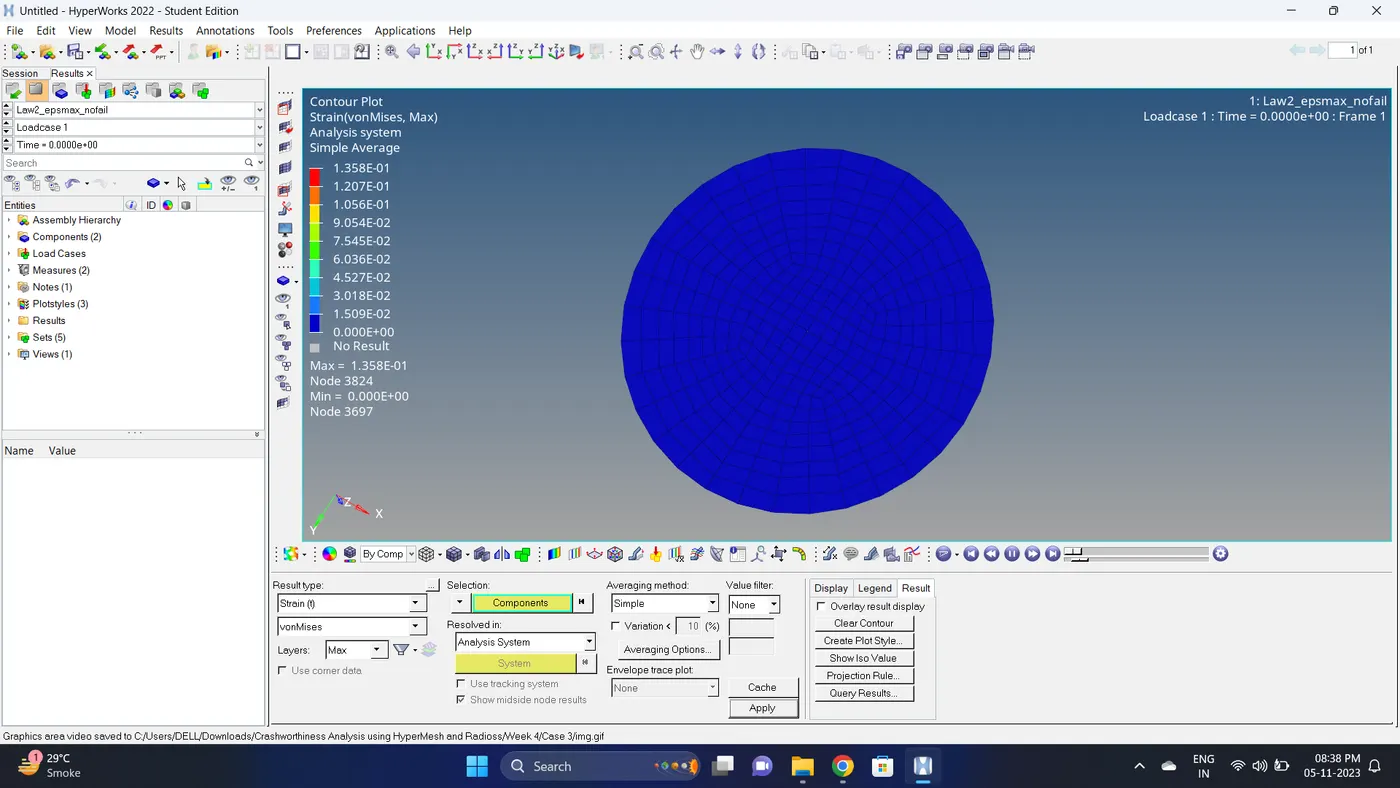
10. Go to the contour - change result type to strain (t), averaging method to simple, click on apply and play the animation.
Maximum strain = 0.1358 and Minimum stain is 0
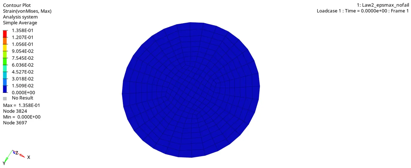
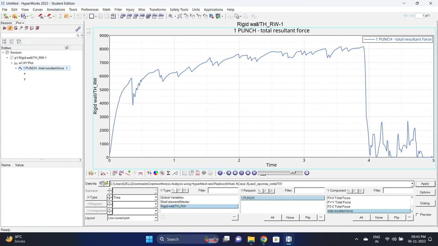
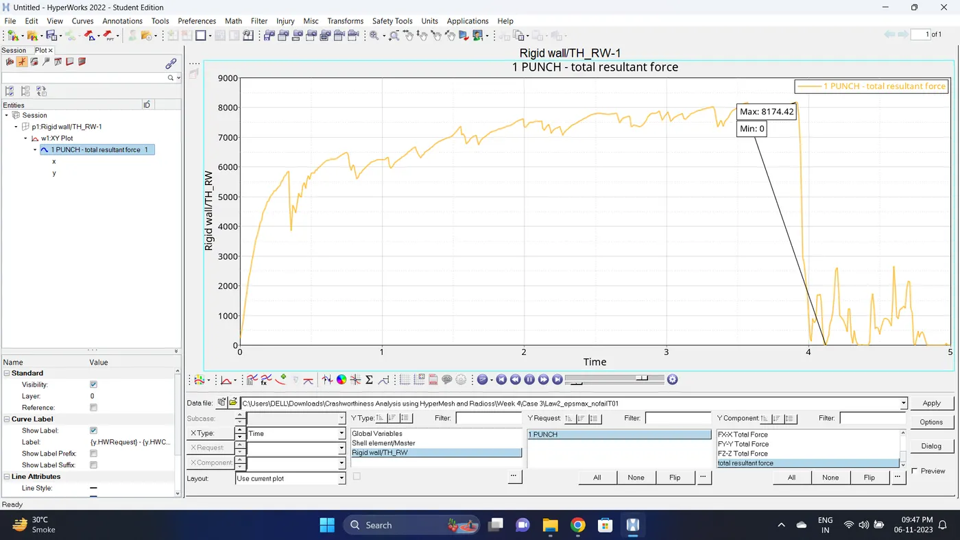
11. Plot the rigid wall forces.
Case 4
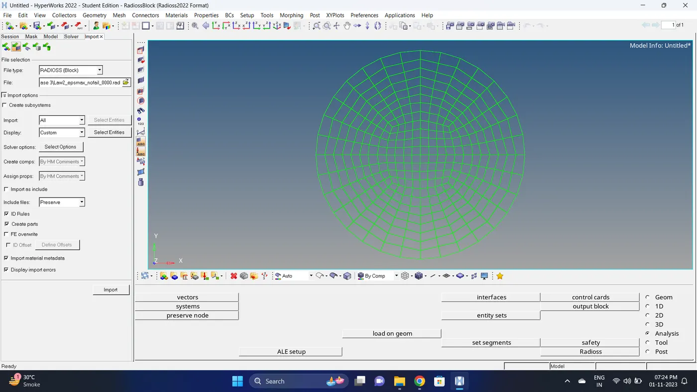
1. Import the case 3 rad file, named “Law2_epsmax_nofail”.
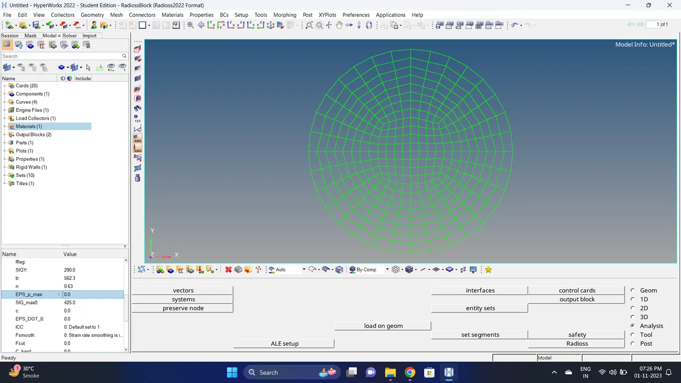
2. Change the EPS_p_max value to 0.
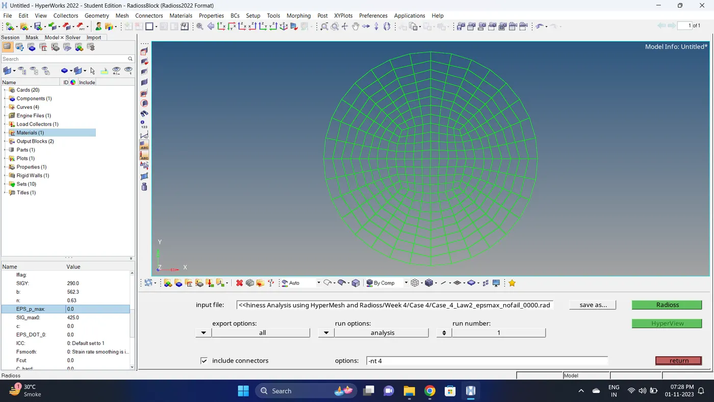
3. Run the simulation
Go to Analysis - Radioss - click on save as, Rename the file to Case_4_Law2_epsmax_nofail and at the end type .rad - Ensure that export option is set to all and Include connectors is tick - Click Radioss to run the simulation.
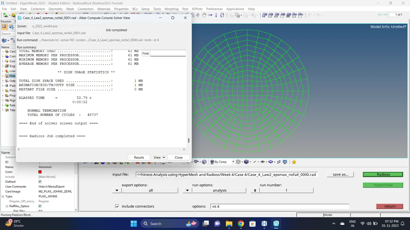
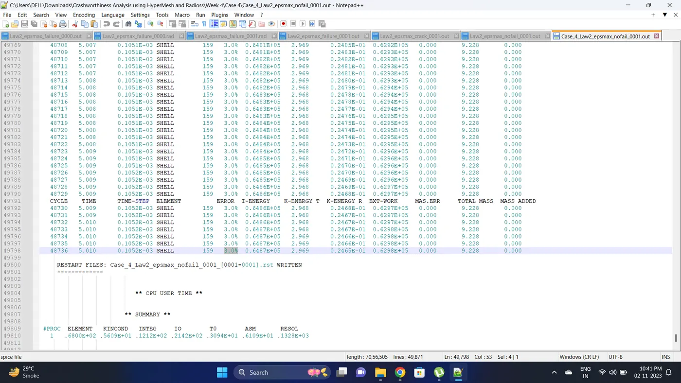
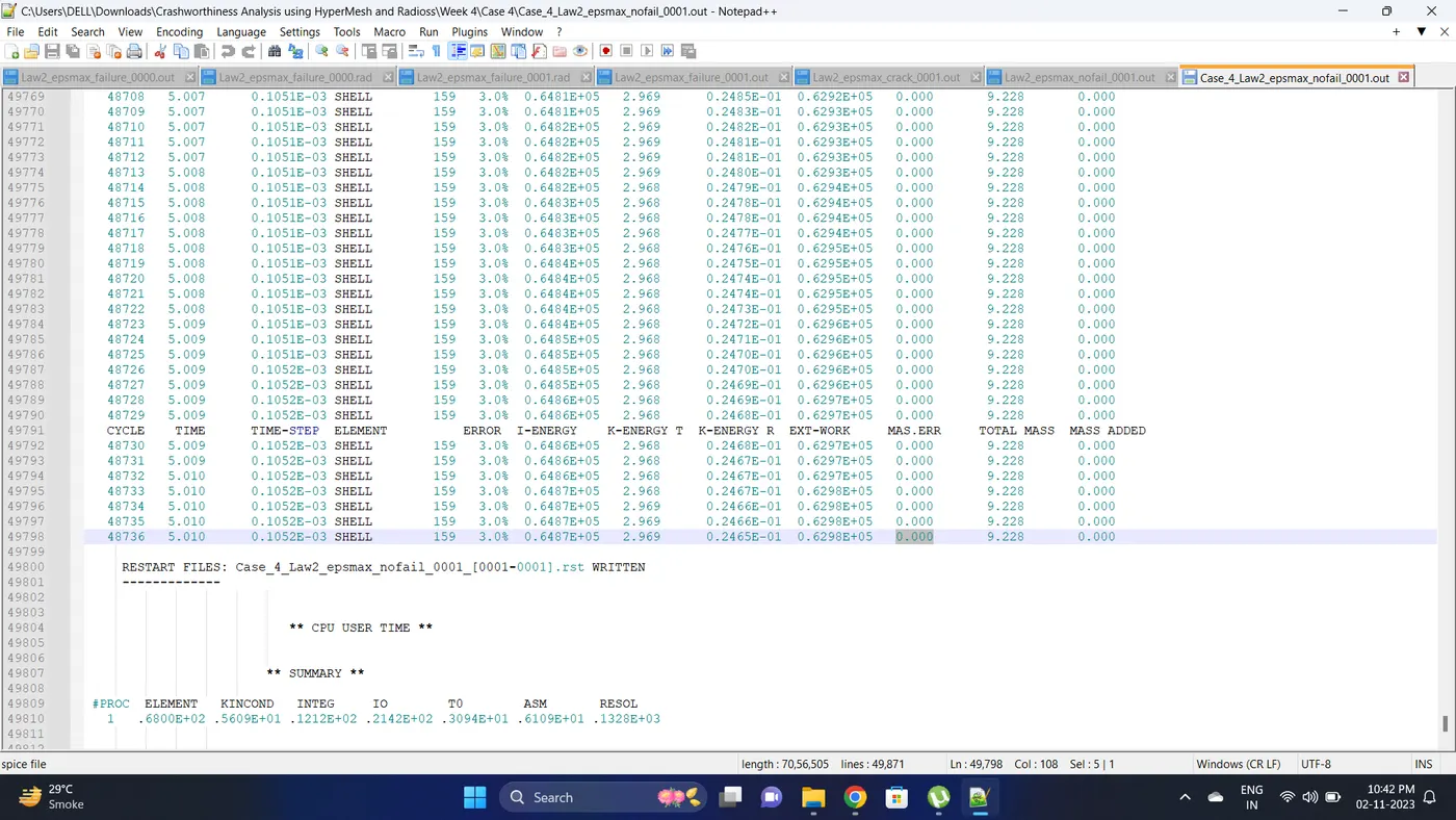
4. Open 0001.out file in notepad ++ and check the maximum total energy error and mass error.
The torelance for the energy error is -15 to +5 % and mass error is upto 2 %
Energy error is 3 %
Mass error is 0 %
5. Open the Hyperwork in Hypergraph 2D view.
6. Open the T01 file from case_4 and select the Global Variable - Internal energy, Kinetic energy, Contact Energy, Hourglass Energy and Total Energy - Click apply to plot the graph.
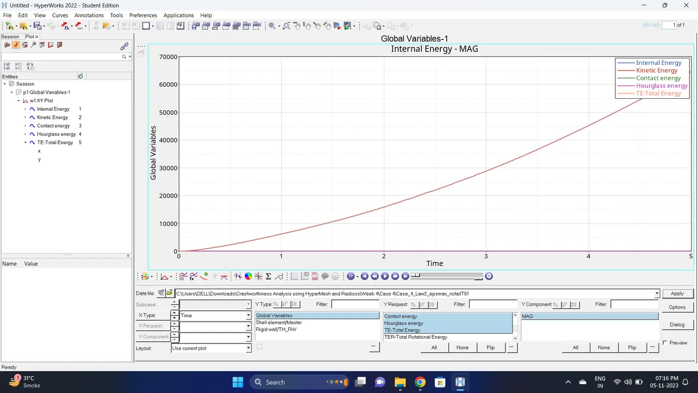
7. Note down the minimum and maximum value of various Energy by right click on any energy - Single curve math - Min Note. similarly do for maximum
Note: after getting graph reading turn off that graph and do next reading.
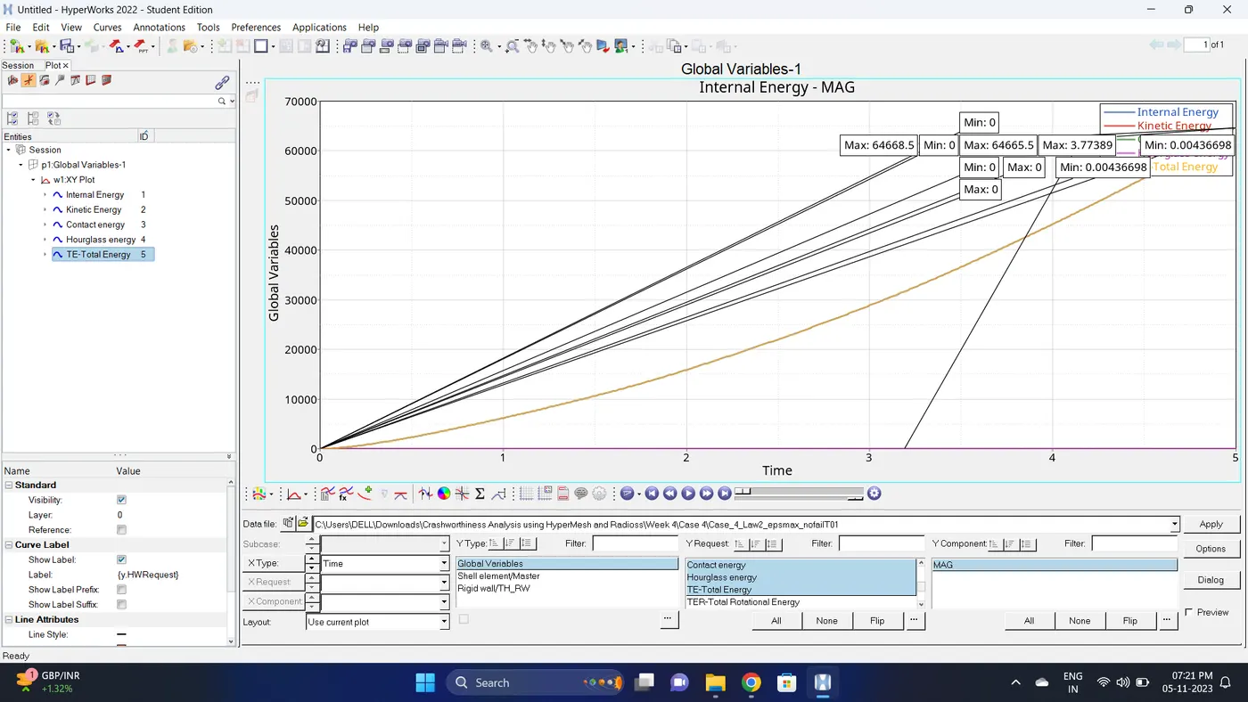
| Sr.no | Name | Minimum | Maximum |
| 1 | Internal Energy | 0 | 64665.5 |
| 2 | Kinetic Energy | 0.00436698 | 3.77389 |
| 3 | Contact Energy | 0 | 0 |
| 4 | Hourglass Energy | 0 | 0 |
| 5 | Total Energy | 0.00436698 | 64668.5 |
8. Open the Hyperwork in Hyperview view.
9. Import the .h3d file.
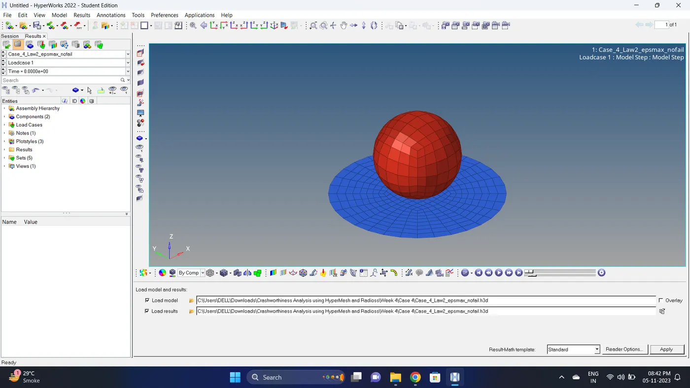
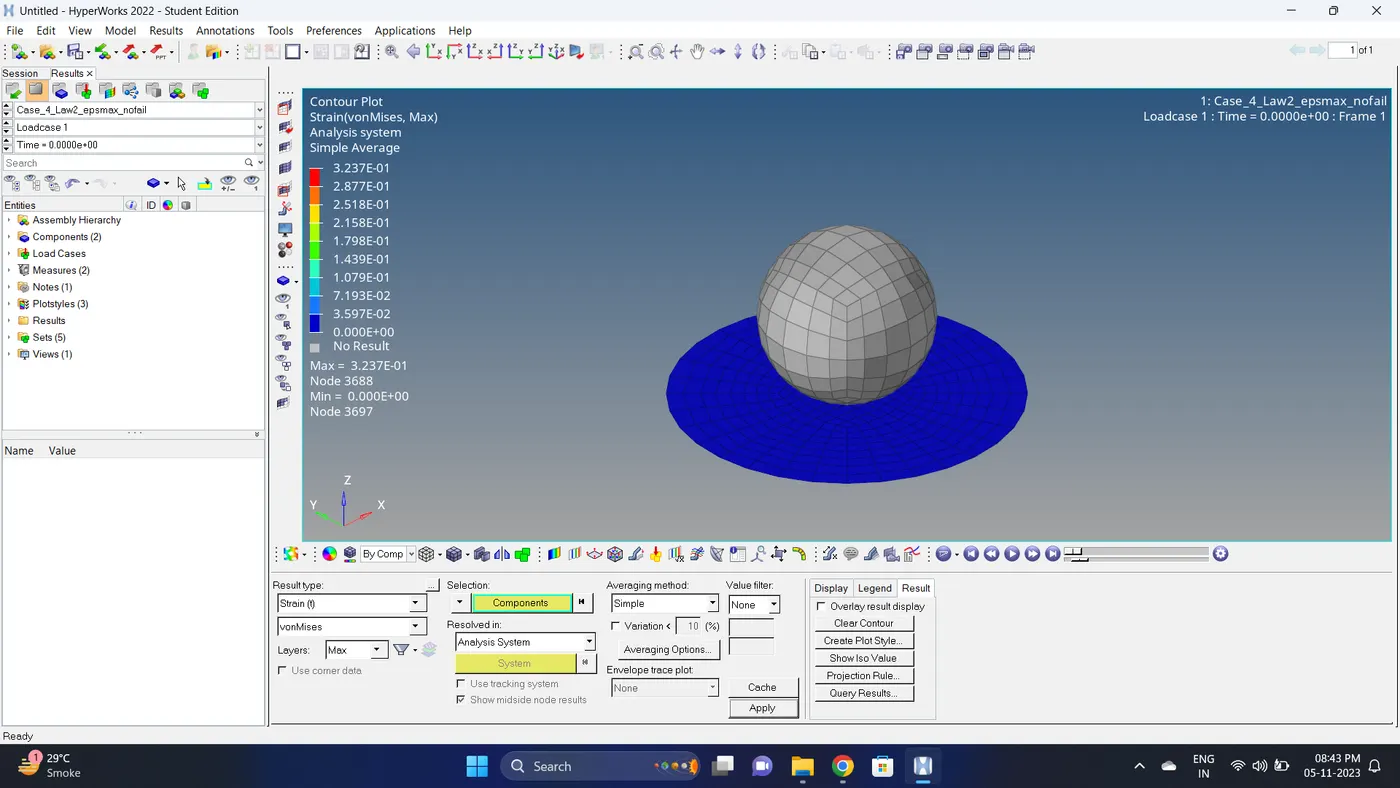
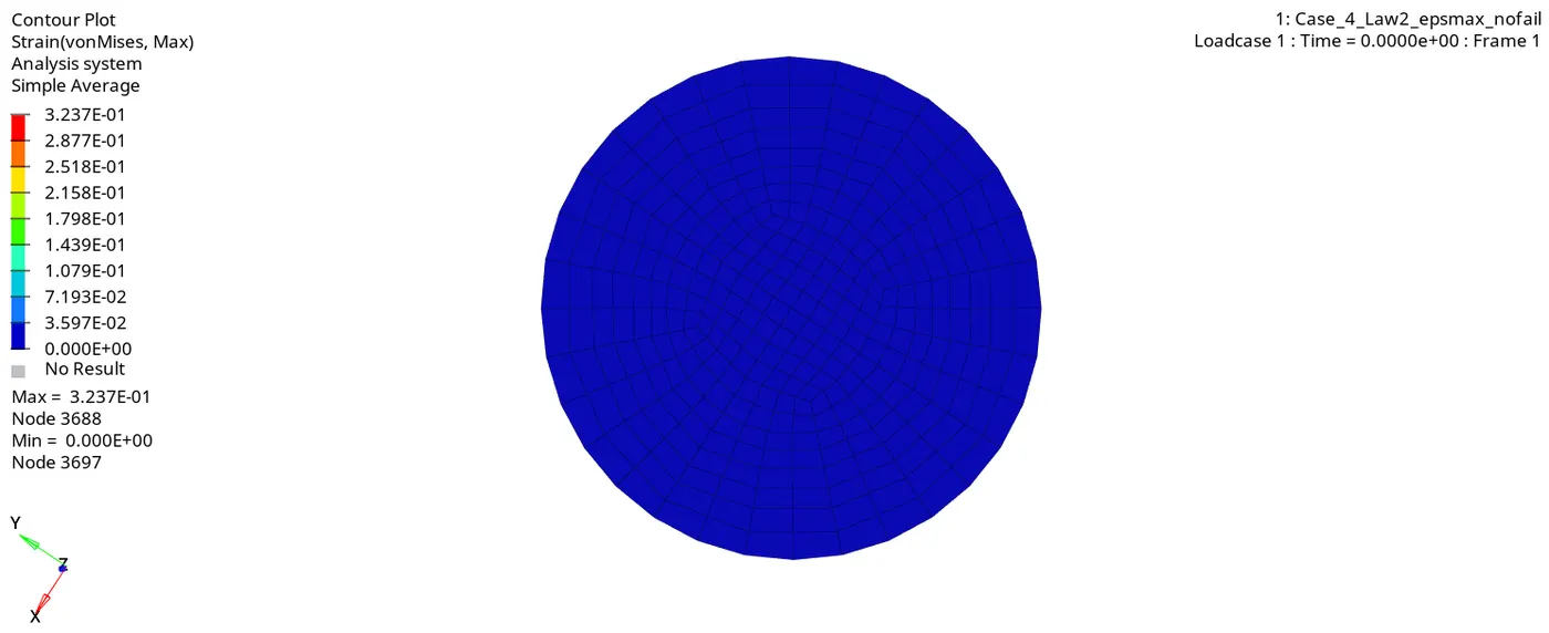
10. Go to the contour - change result type to strain (t), averaging method to simple, click on apply and play the animation.
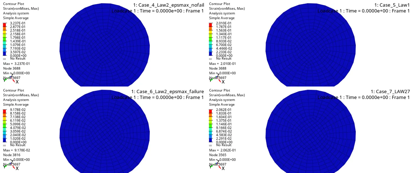
Maximum strain = 0.3237 and Minimum stain is 0
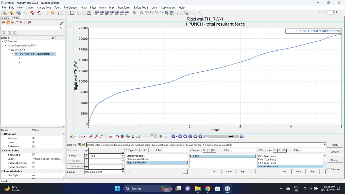
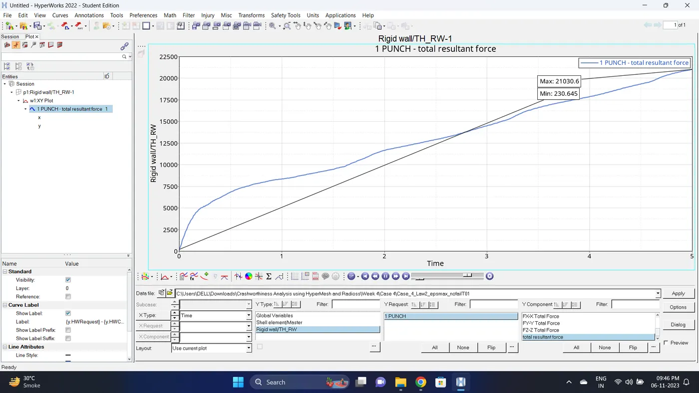
11. Plot the rigid wall forces.
Case 5
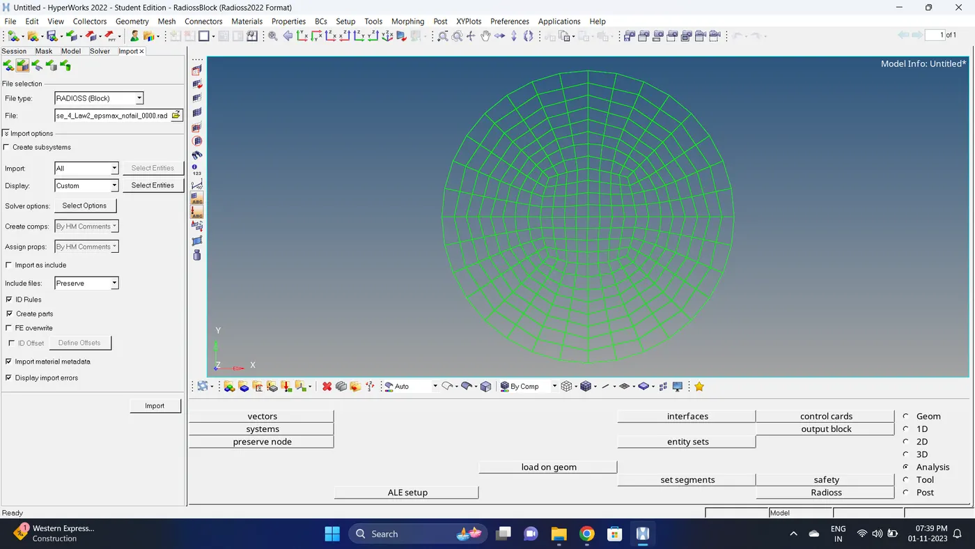
1. Import the case 4 rad file named Case_4_Law2_epsmax_nofail.
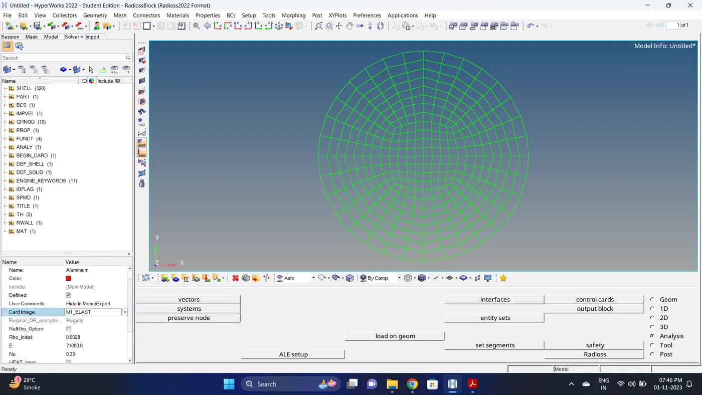
2. Change the material card to Law 1. Keep the same value for rho, E, and nu values.
3. Run the simulation
Go to Analysis - Radioss - click on save as, Rename the file to Case_5_Law1 and at the end type .rad - Ensure that export option is set to all and Include connectors is tick - Click Radioss to run the simulation.
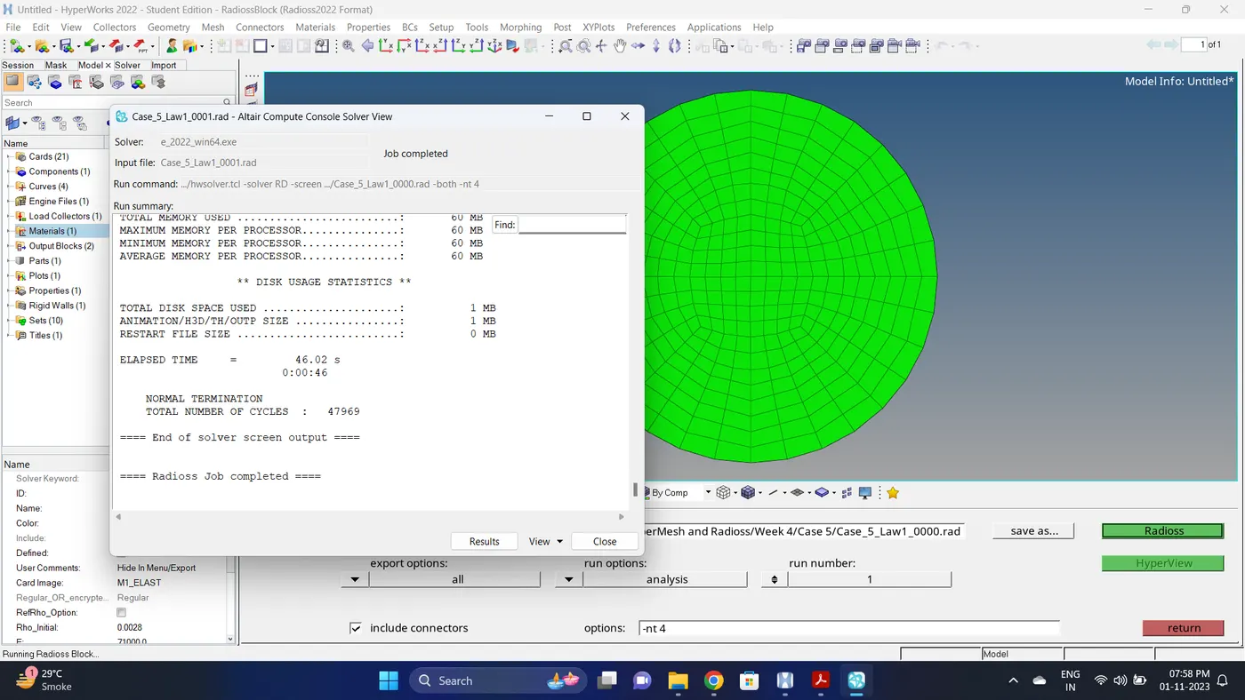
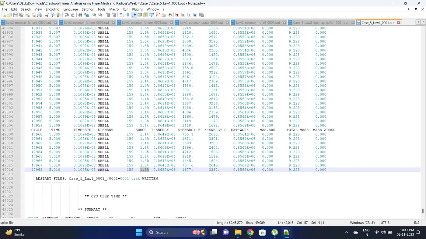
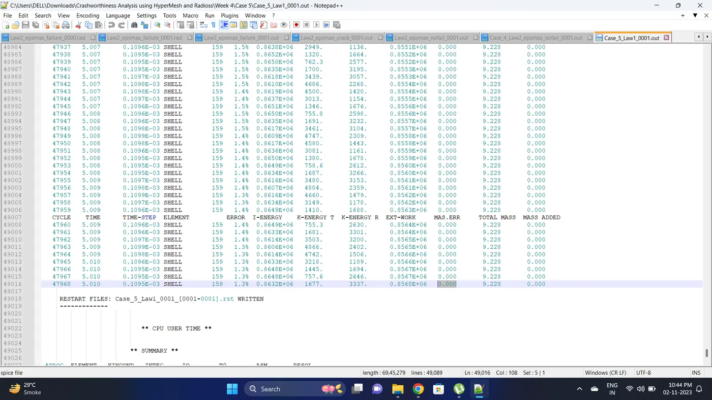
4. Open 0001.out file in notepad ++ and check the maximum total energy error and mass error.
The torelance for the energy error is -15 to +5 % and mass error is upto 2 %
Energy error is 1.3 %
Mass error is 0 %
5. Open the Hyperwork in Hypergraph 2D view.
6. Open the T01 file from case_5 and select the Global Variable - Internal energy, Kinetic energy, Contact Energy, Hourglass Energy and Total Energy - Click apply to plot the graph.
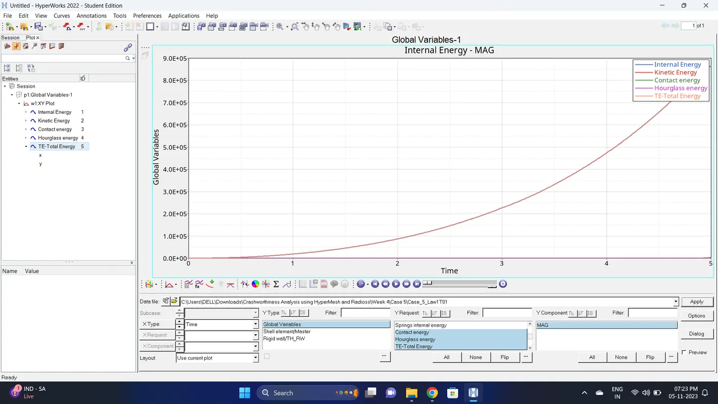
7. Note down the minimum and maximum value of various Energy by right click on any energy - Single curve math - Min Note. similarly do for maximum
Note: after getting graph reading turn off that graph and do next reading.
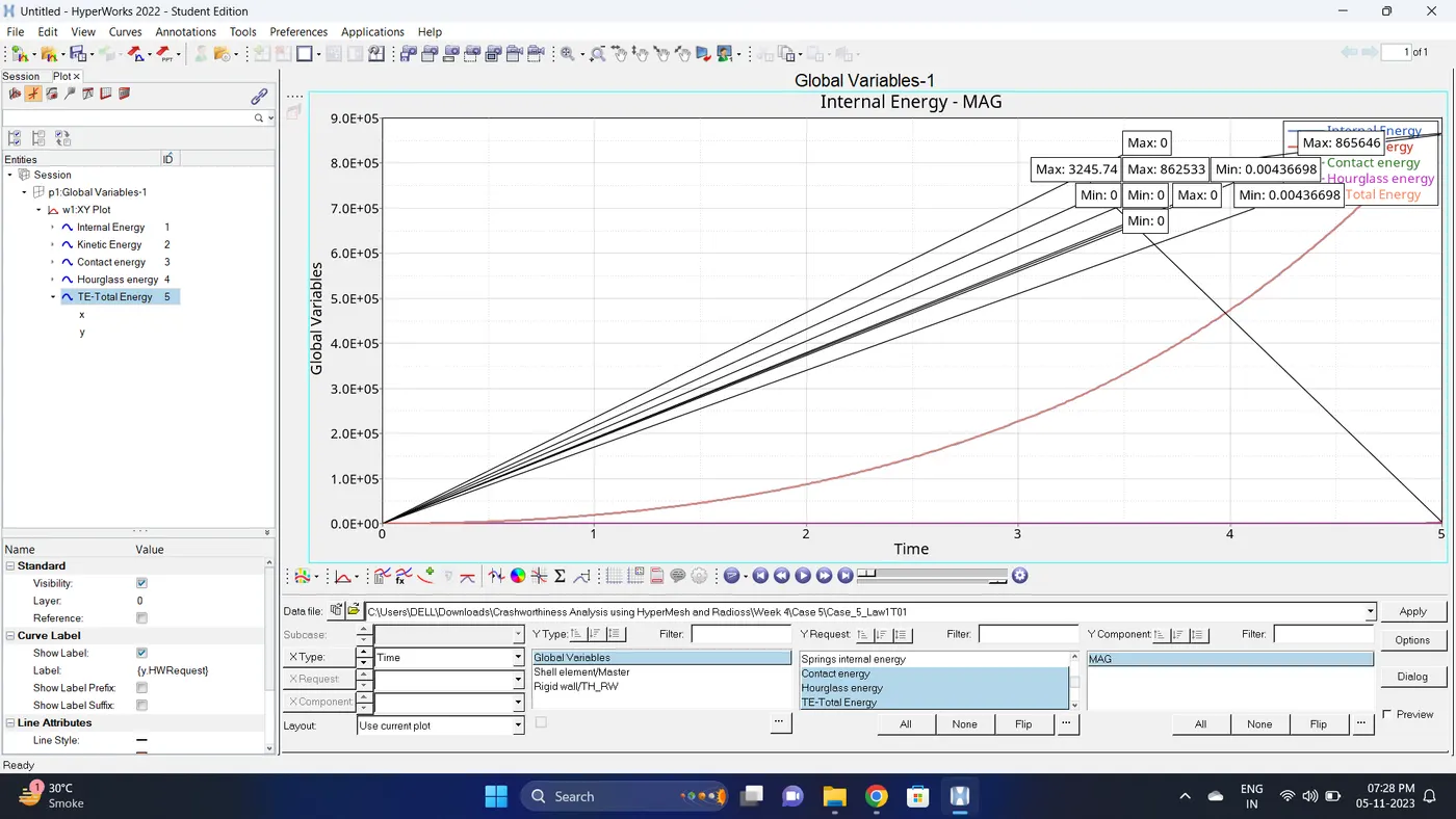
| Sr.no | Name | Minimum | Maximum |
| 1 | Internal Energy | 0 | 862533 |
| 2 | Kinetic Energy | 0.00436698 | 3245.74 |
| 3 | Contact Energy | 0 | 0 |
| 4 | Hourglass Energy | 0 | 0 |
| 5 | Total Energy | 0.00436698 | 865646 |
8. Open the Hyperwork in Hyperview view.
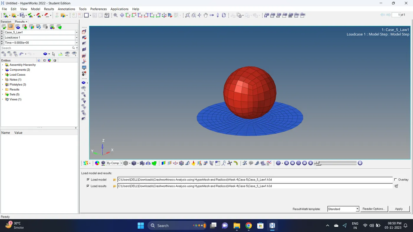
9. Import the .h3d file.
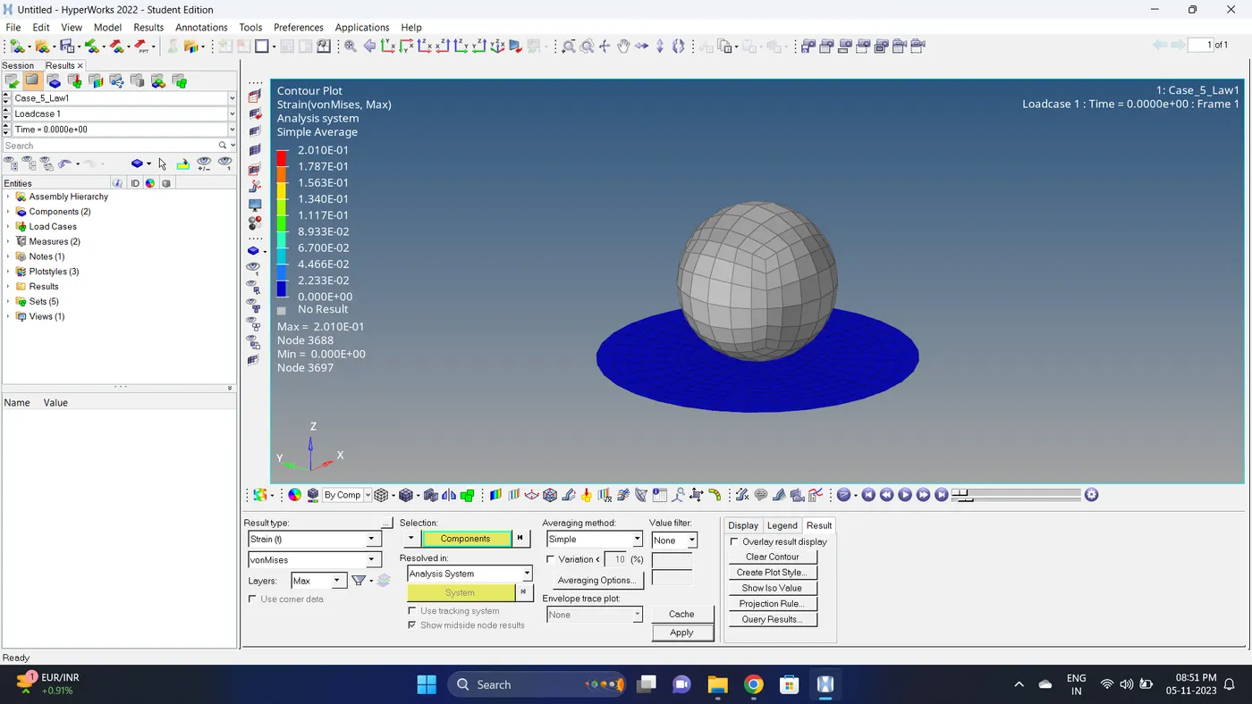
9. Go to the contour - change result type to strain (t), averaging method to simple, click on apply and play the animation.
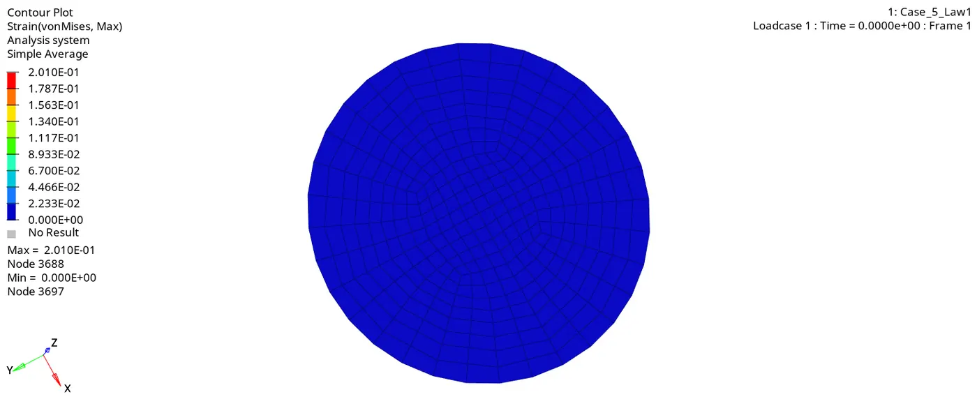
Maximum strain = 0.2010 and Minimum stain is 0
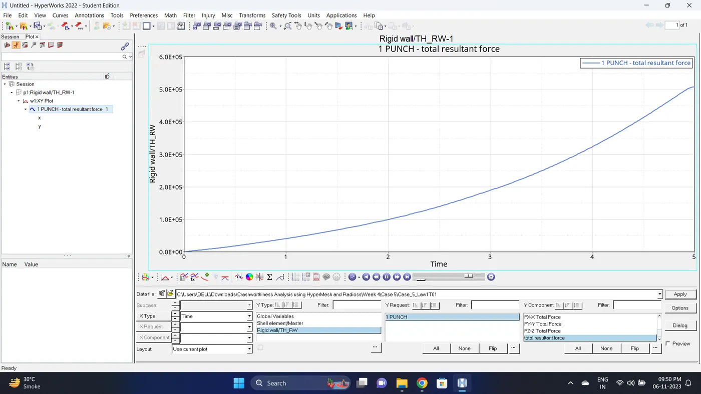
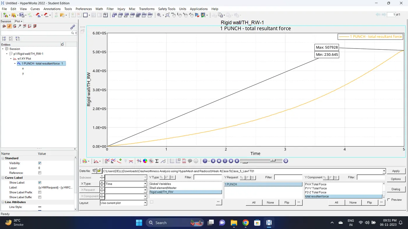
10. Plot the rigid wall forces.
Case 6
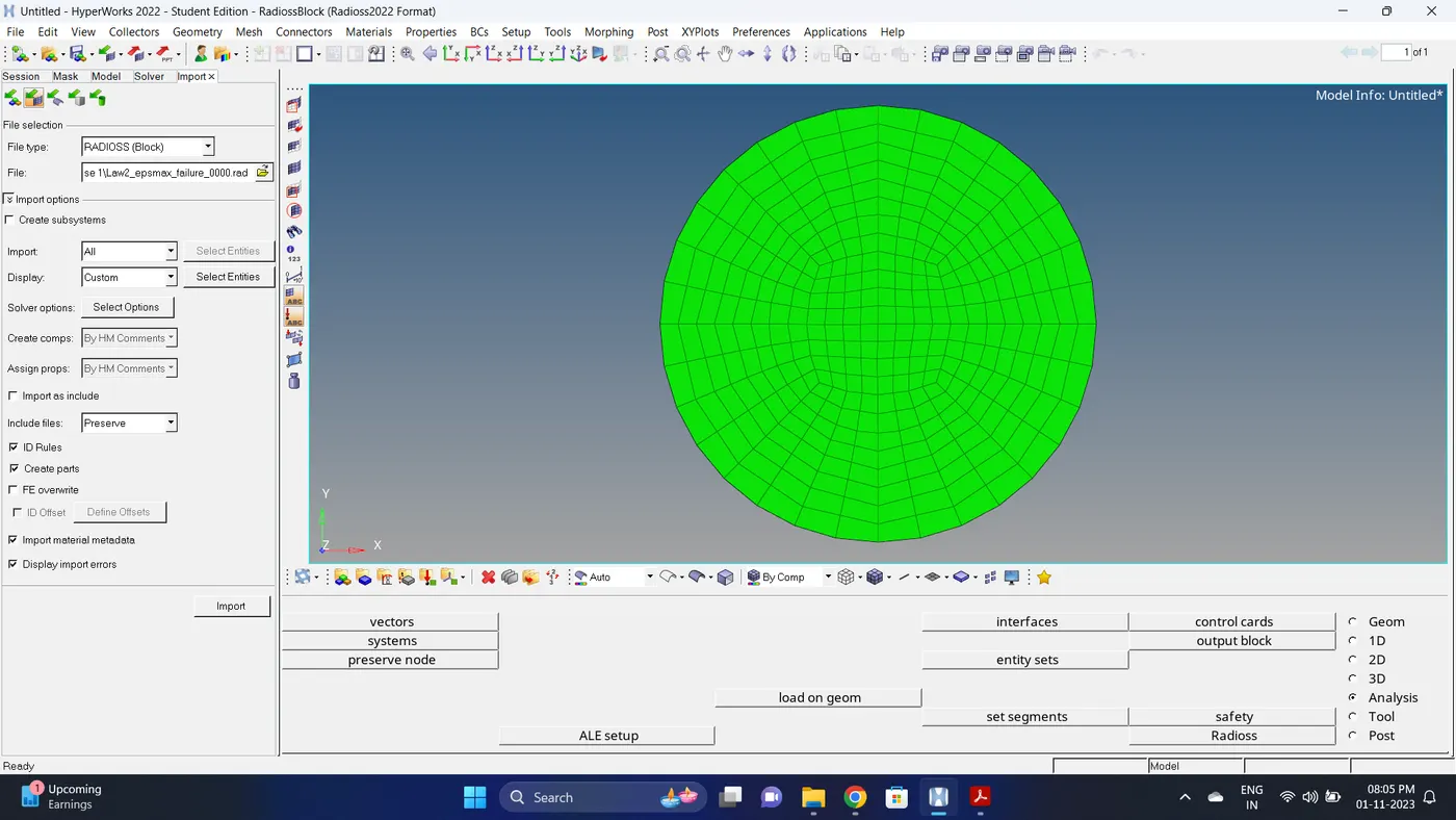
1. Import the case 1 rad file, named “Law2_epsmax_failure”.
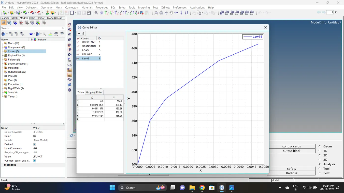
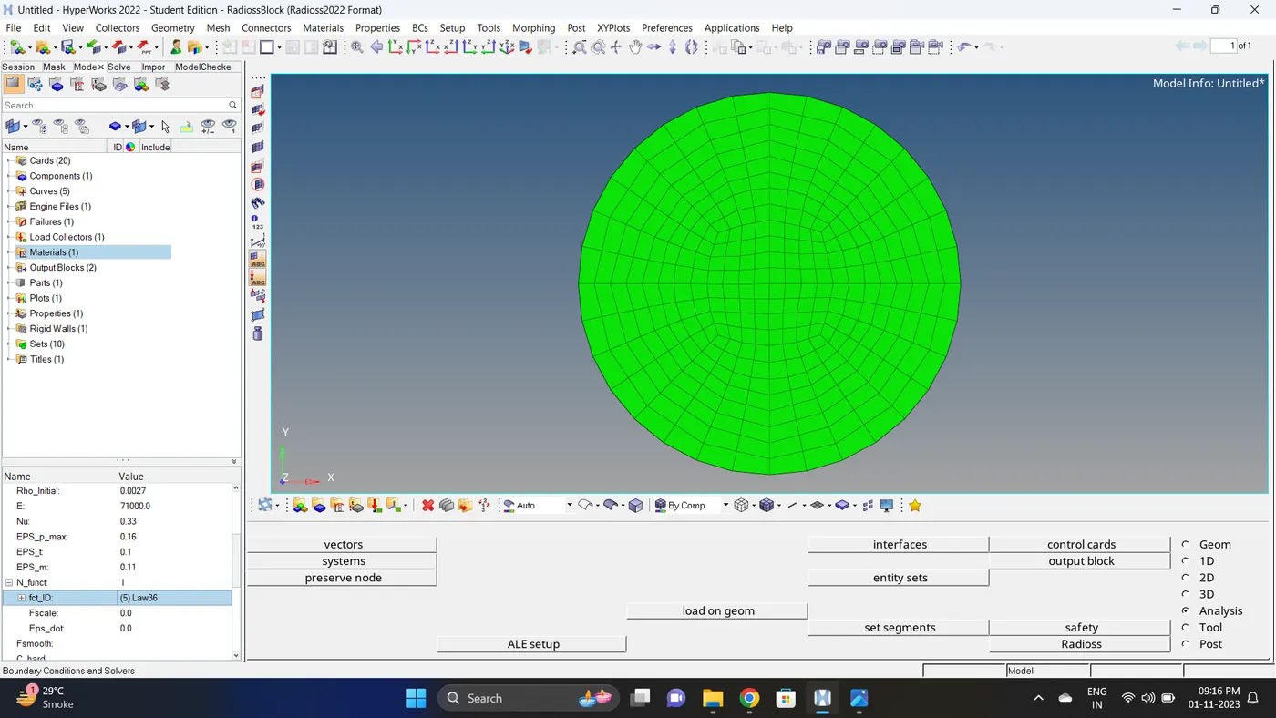
2. Change the material card to law 36_Plas_Tab and give material property as given.
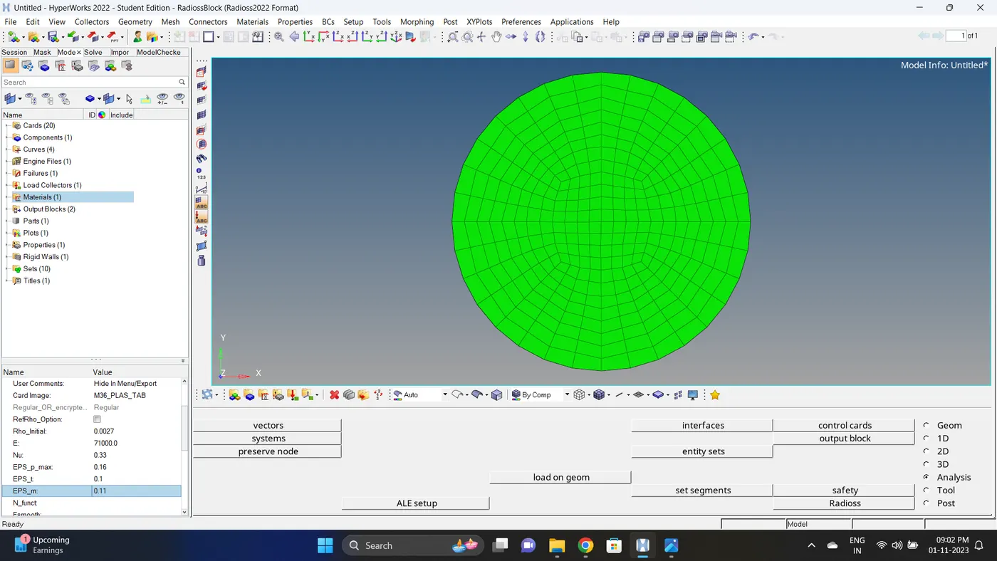
3. Plot the curve as the information given in the video and then select that curve in the N_funct.
4. Run the simulation
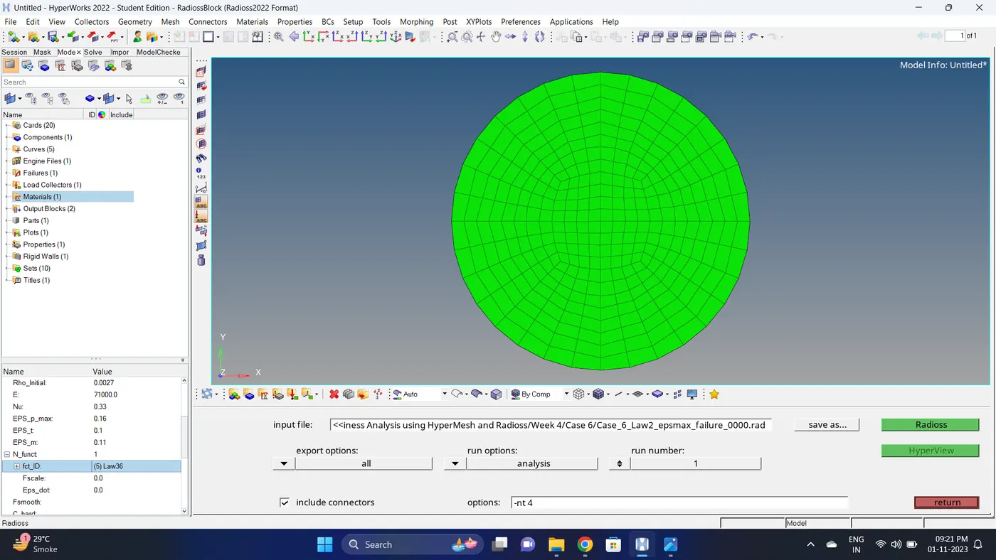
Go to Analysis - Radioss - click on save as, Rename the file to Case_5_Law1 and at the end type .rad - Ensure that export option is set to all and Include connectors is tick - Click Radioss to run the simulation.
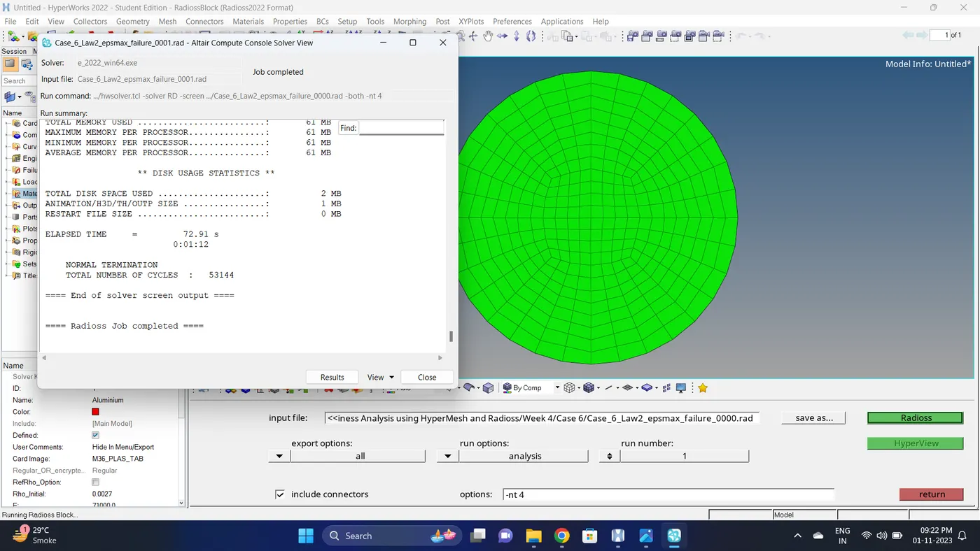
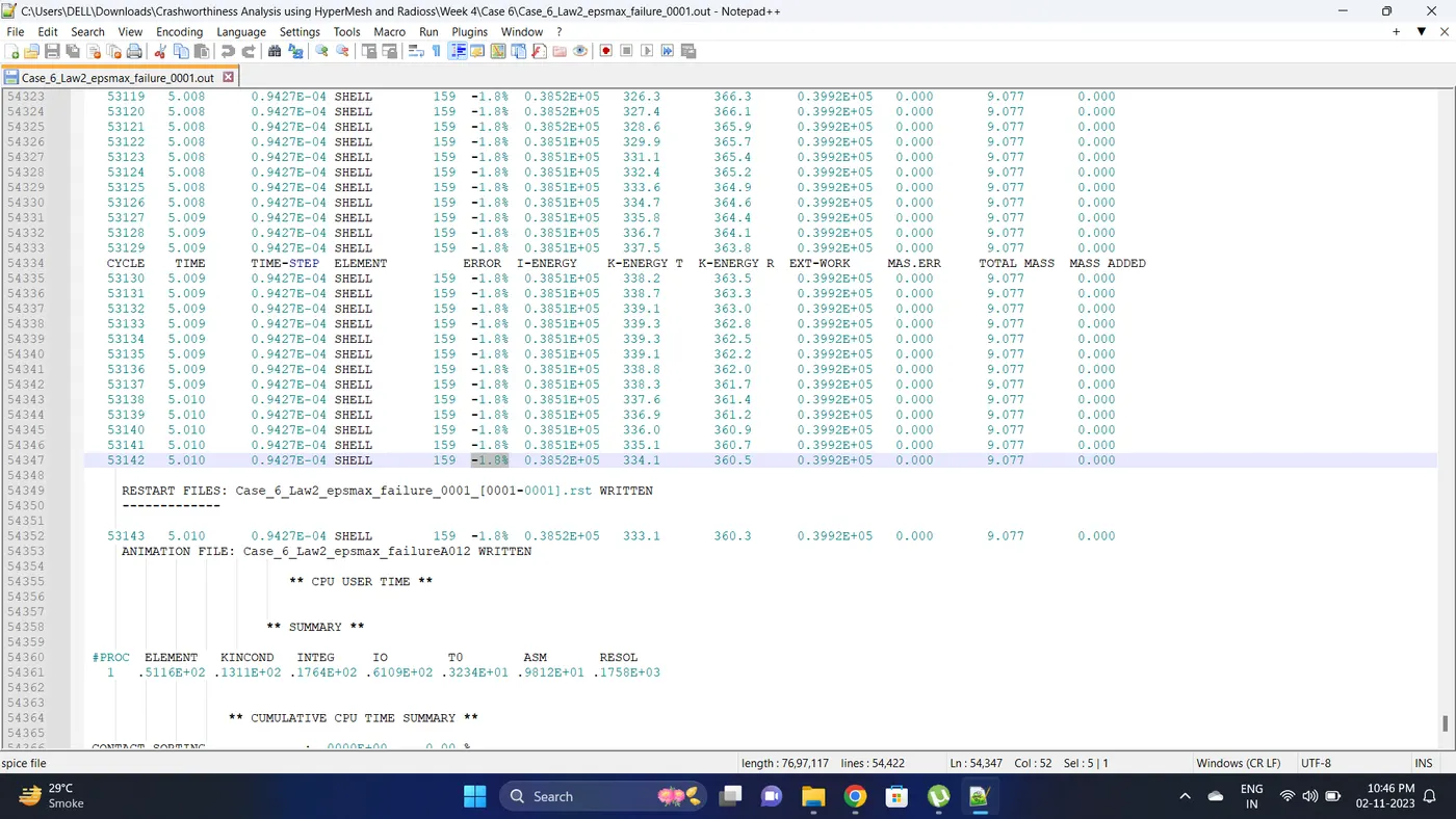
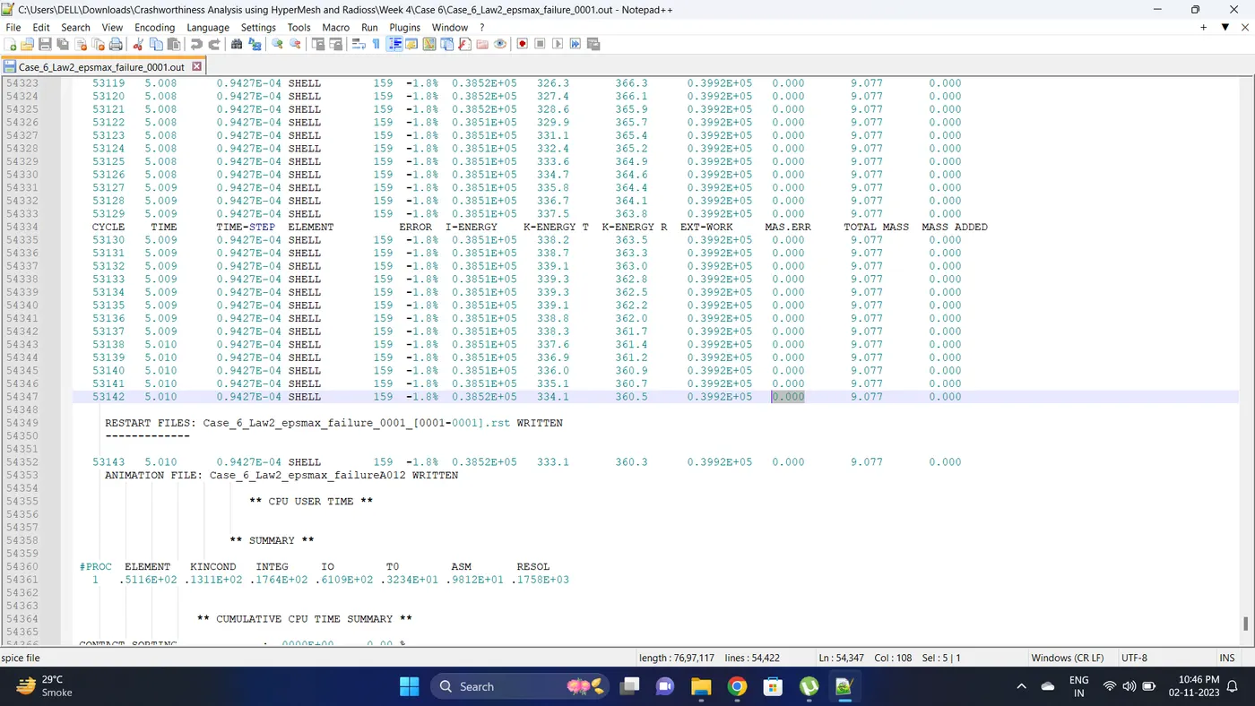
5. Open 0001.out file in notepad ++ and check the maximum total energy error and mass error.
The torelance for the energy error is -15 to +5 % and mass error is upto 2 %
Energy error is -1.8 %
Mass error is 0 %
6. Open the Hyperwork in Hypergraph 2D view.
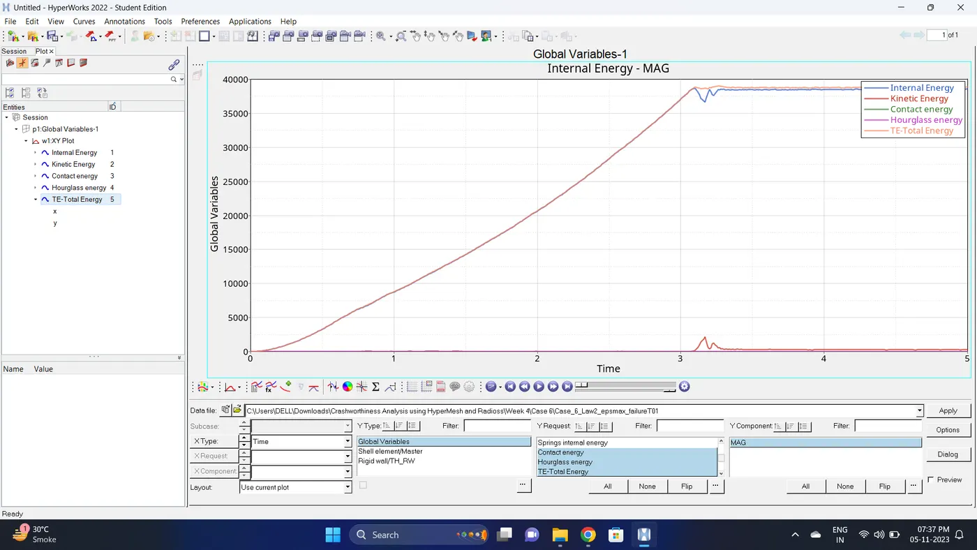
7. Open the T01 file from case_6 and select the Global Variable - Internal energy, Kinetic energy, Contact Energy, Hourglass Energy and Total Energy - Click apply to plot the graph.
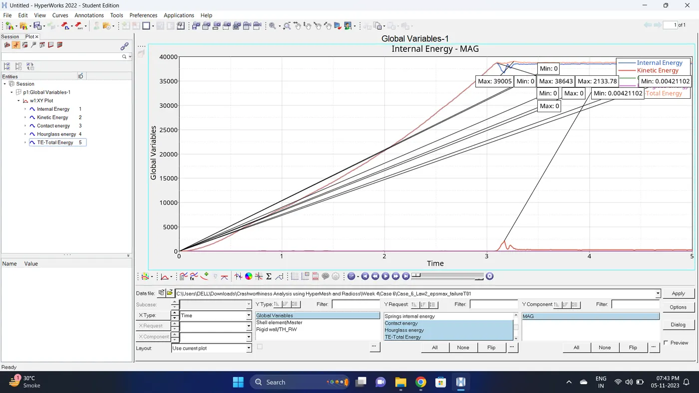
8. Note down the minimum and maximum value of various Energy by right click on any energy - Single curve math - Min Note. similarly do for maximum
Note: after getting graph reading turn off that graph and do next reading.
| Sr.no | Name | Minimum | Maximum |
| 1 | Internal Energy | 0 | 38643 |
| 2 | Kinetic Energy | 0.00421102 | 2133.78 |
| 3 | Contact Energy | 0 | 0 |
| 4 | Hourglass Energy | 0 | 0 |
| 5 | Total Energy | 0.00421102 | 39005 |
9. Open the Hyperwork in Hyperview view.
10. Import the .h3d file.
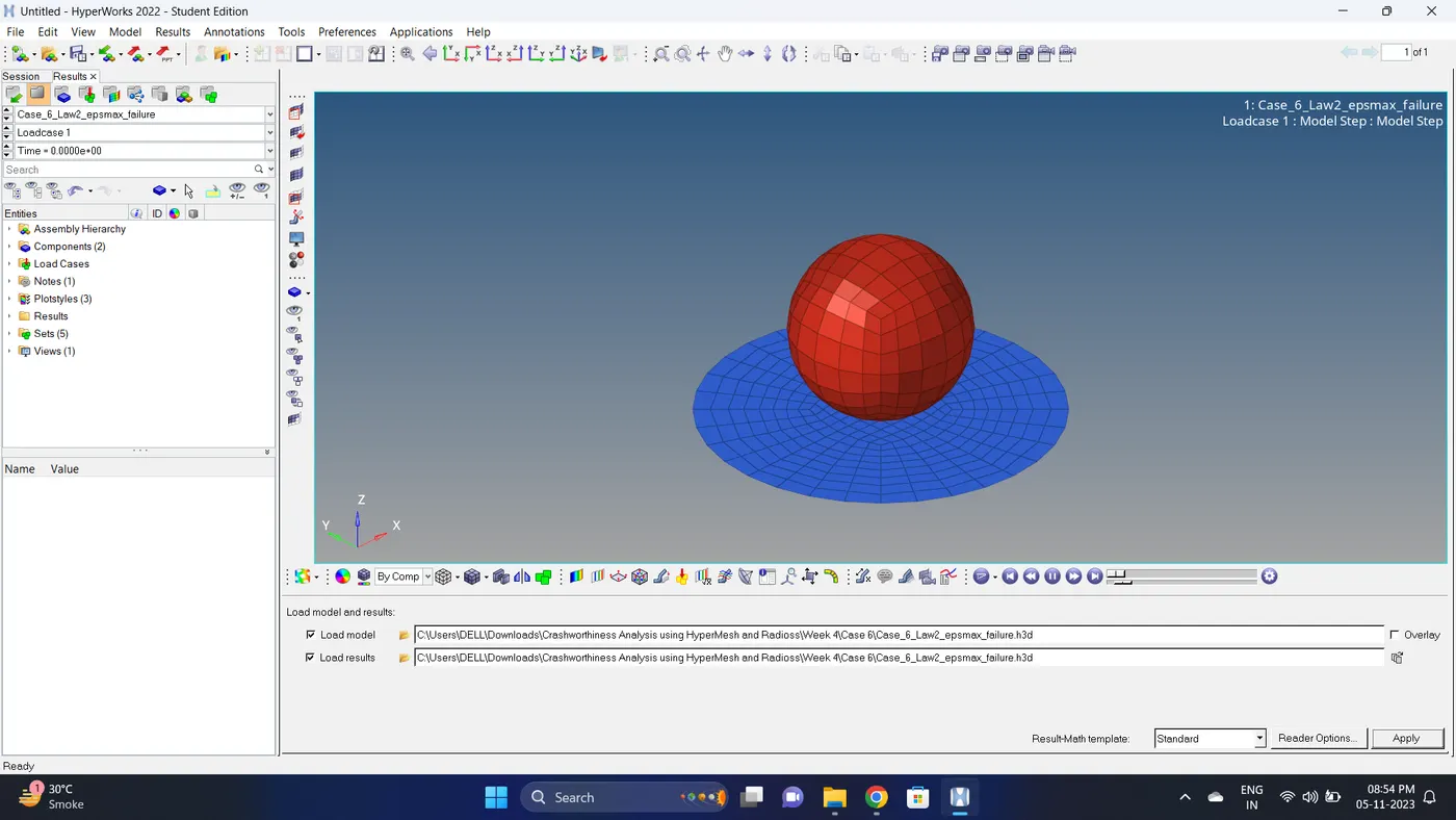
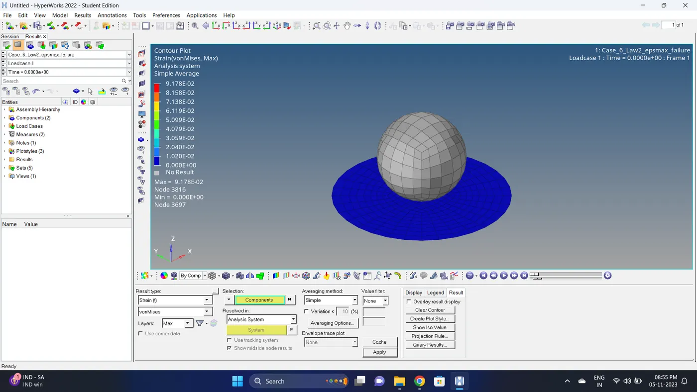
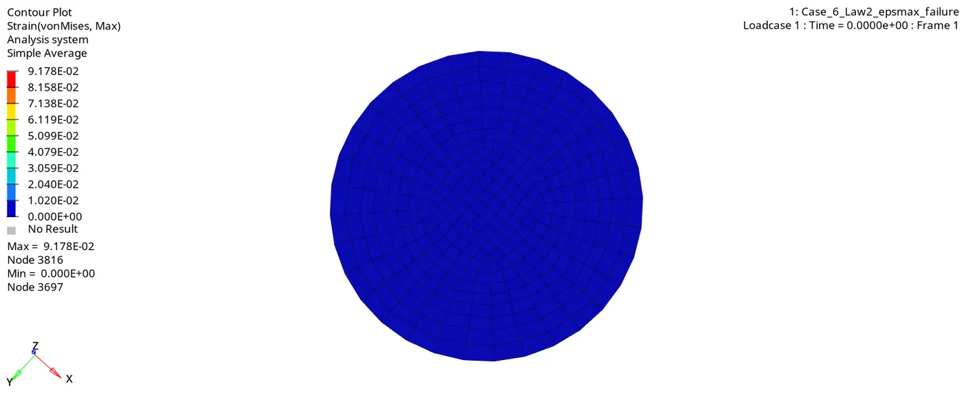
11. Go to the contour - change result type to strain (t), averaging method to simple, click on apply and play the animation.
Maximum strain = 0.09178 and Minimum stain is 0
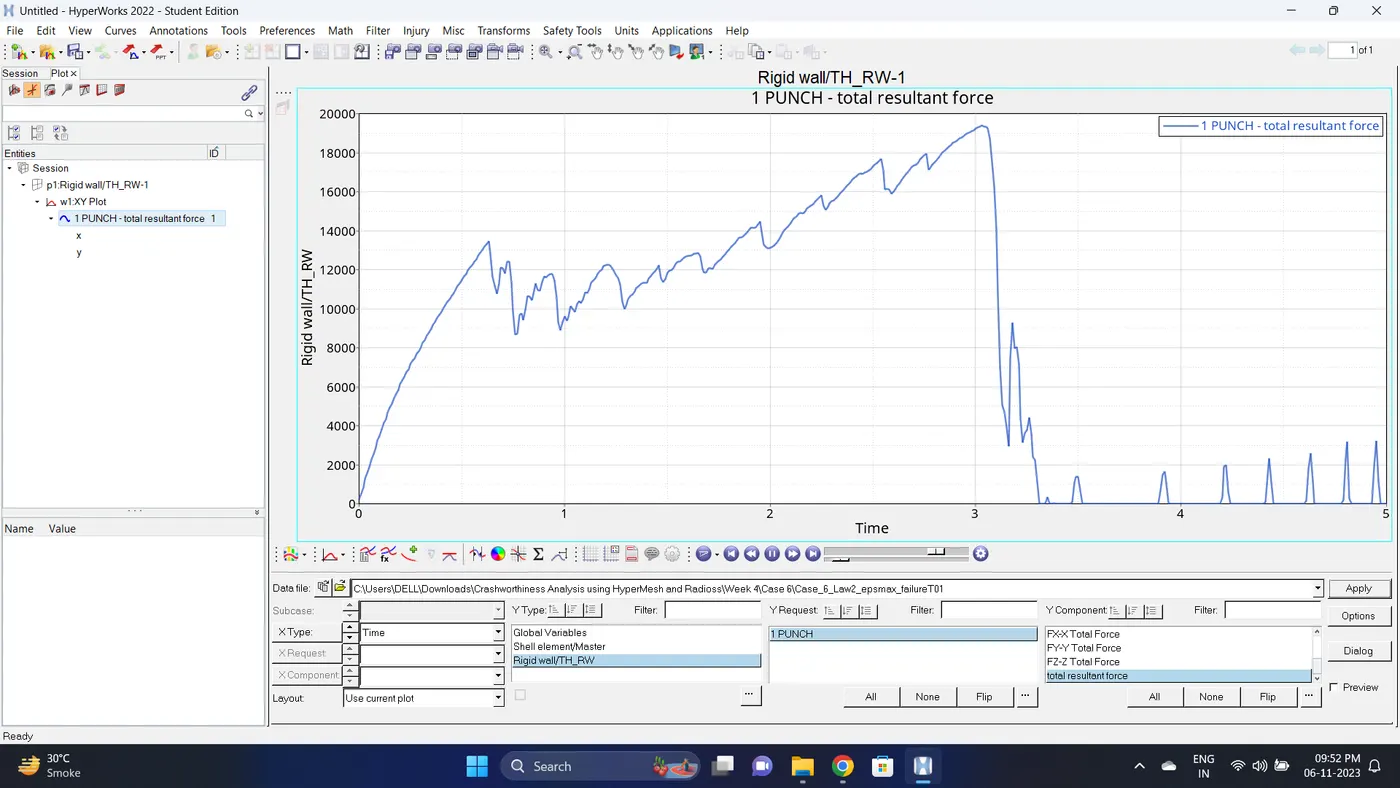
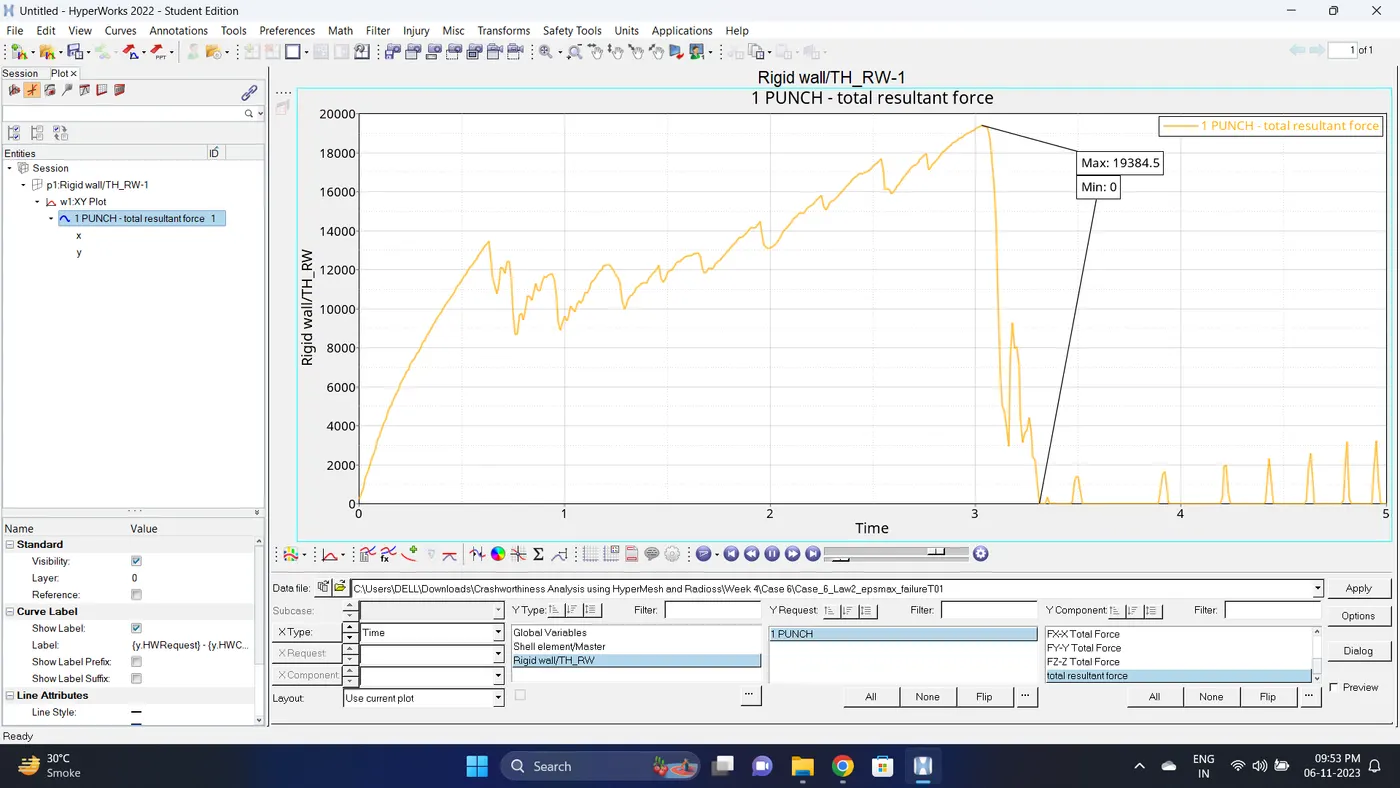
12. Plot the rigid wall forces.
Case 7
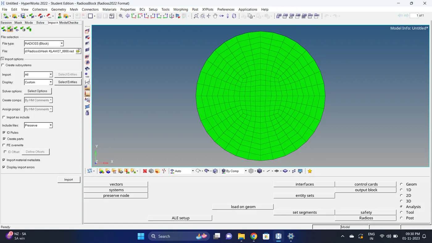
1. Import the Law27_0000.rad file.
2. Run the simulation
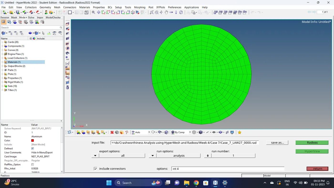
Go to Analysis - Radioss - click on save as, Rename the file to Case_7_LAW27 and at the end type .rad - Ensure that export option is set to all and Include connectors is tick - Click Radioss to run the simulation.
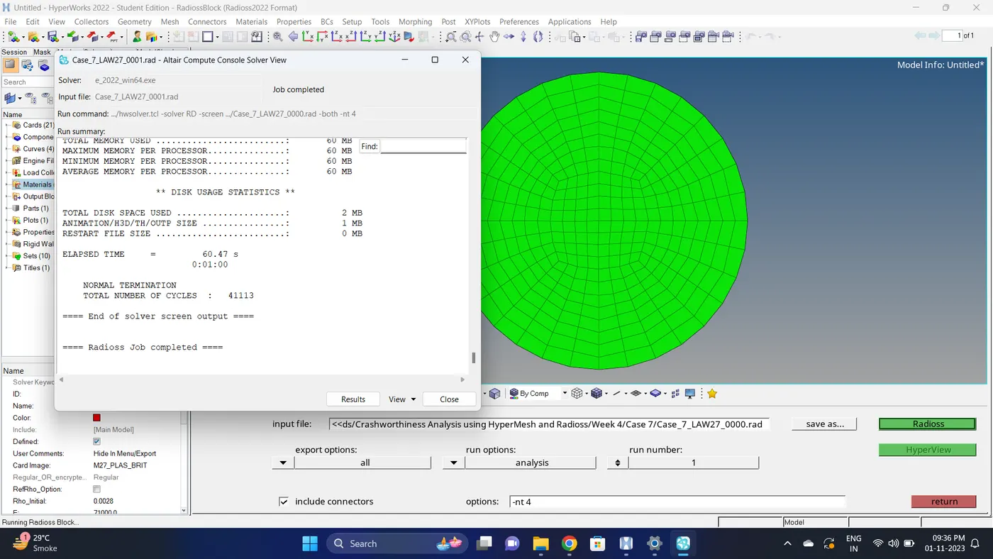
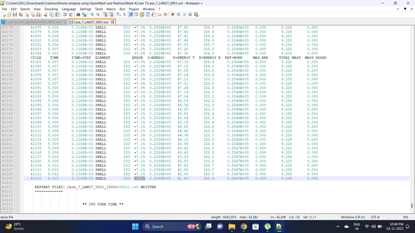
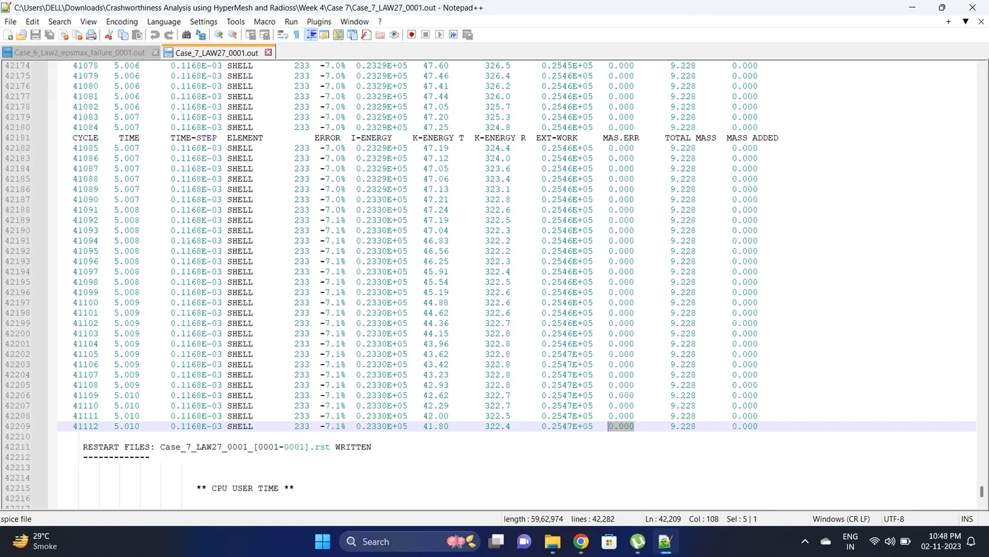
3. Open 0001.out file in notepad ++ and check the maximum total energy error and mass error.
The torelance for the energy error is -15 to +5 % and mass error is upto 2 %
Energy error is -7.1 %
Mass error is 0 %
4. Open the Hyperwork in Hypergraph 2D view.
5. Open the T01 file from case_7 and select the Global Variable - Internal energy, Kinetic energy, Contact Energy, Hourglass Energy and Total Energy - Click apply to plot the graph.
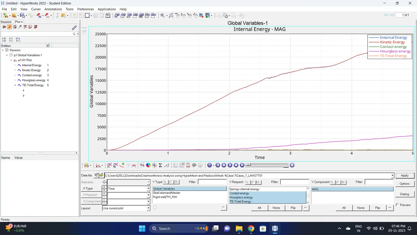
6. Note down the minimum and maximum value of various Energy by right click on any energy - Single curve math - Min Note. similarly do for maximum
Note: after getting graph reading turn off that graph and do next reading.
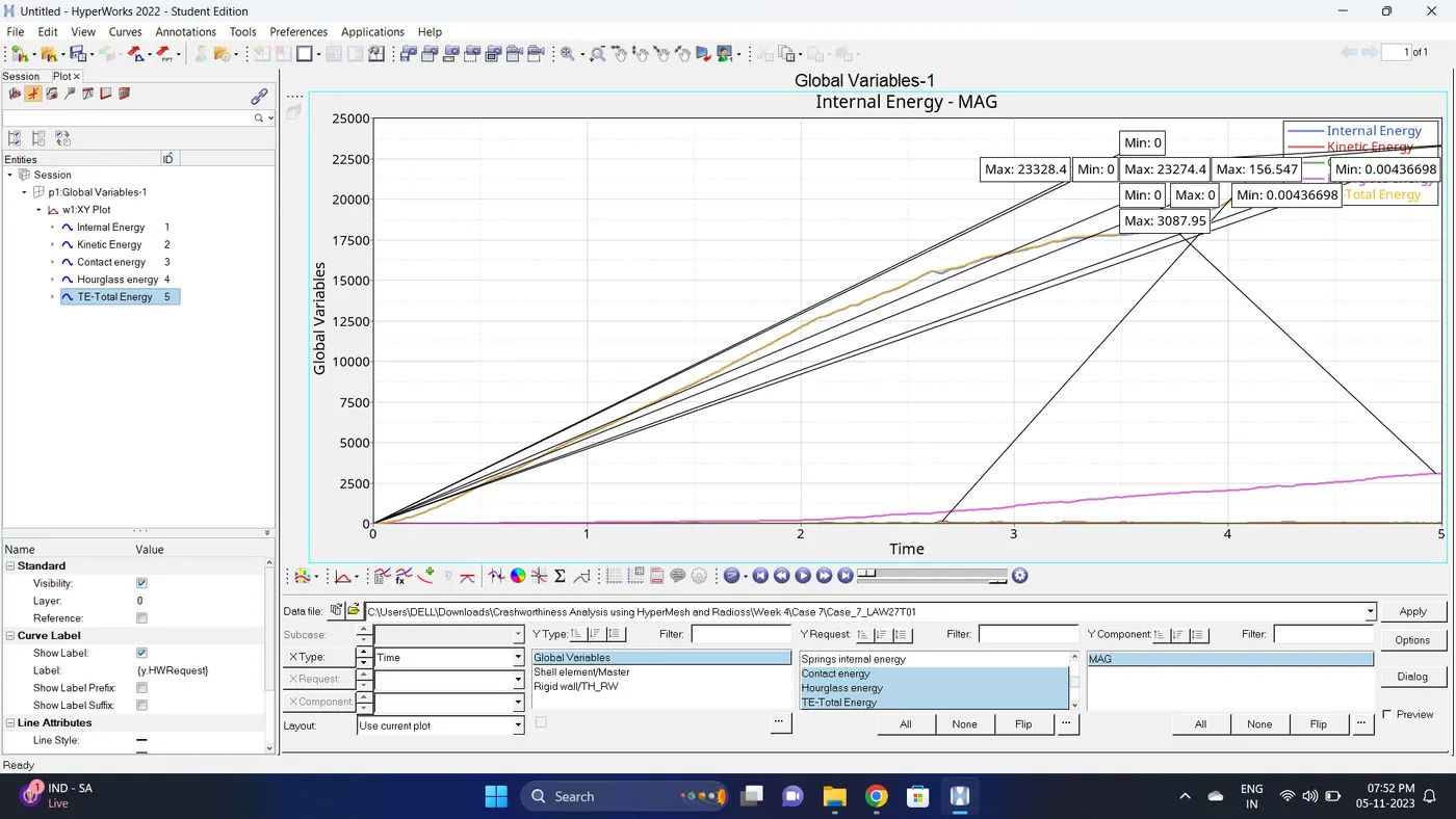
| Sr.no | Name | Minimum | Maximum |
| 1 | Internal Energy | 0 | 23274.4 |
| 2 | Kinetic Energy | 0.00436698 | 156.547 |
| 3 | Contact Energy | 0 | 0 |
| 4 | Hourglass Energy | 0 | 3087.95 |
| 5 | Total Energy | 0.00436698 | 23328.4 |
7. Open the Hyperwork in Hyperview view.
8. Import the .h3d file.
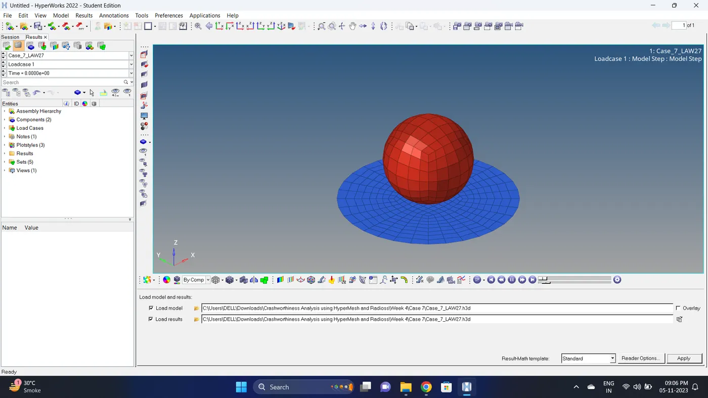
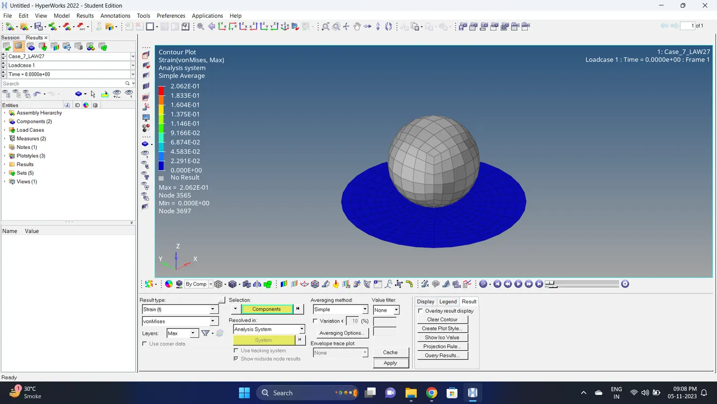
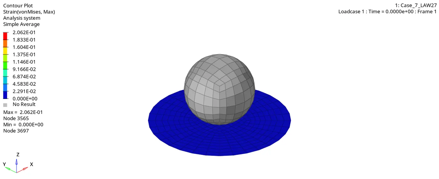
9. Go to the contour - change result type to strain (t), averaging method to simple, click on apply and play the animation.
Maximum strain = 0.2062 and Minimum stain is 0
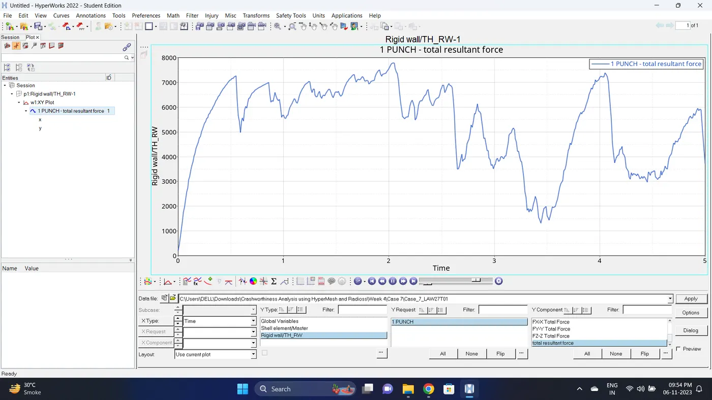
10. Plot the rigid wall forces.
Comparison of Cases:
Comparison between the case 1, 2, 3 and 4:
- In all these 4 cases the Johnson cook material card is used.
- This law represents an isotrpic elastic - plastic material using the Johnson - Cook material model.
- This Model expresses material stress as a function of strain, strain rate and temperature. A build in failure criteria based on the maximum plastic strain is available.
Case 1
| Sr.no | Name | Minimum | Maximum |
| 1 | Internal Energy | 0 | 27322.4 |
| 2 | Kinetic Energy | 0.00436698 | 179.256 |
| 3 | Contact Energy | 0 | 0 |
| 4 | Hourglass Energy | 0 | 0 |
| 5 | Total Energy | 0.00436698 | 27375.9 |
Case 2
| Sr.no | Name | Minimum | Maximum |
| 1 | Internal Energy | 0 | 30812.5 |
| 2 | Kinetic Energy | 0.00436698 | 210.286 |
| 3 | Contact Energy | 0 | 0 |
| 4 | Hourglass Energy | 0 | 0 |
| 5 | Total Energy | 0.00436698 | 30953.4 |
Case 3
| Sr.no | Name | Minimum | Maximum |
| 1 | Internal Energy | 0 | 27443.1 |
| 2 | Kinetic Energy | 0.00436698 | 332.073 |
| 3 | Contact Energy | 0 | 0 |
| 4 | Hourglass Energy | 0 | 0 |
| 5 | Total Energy | 0.00436698 | 27528.4 |
Case 4
| Sr.no | Name | Minimum | Maximum |
| 1 | Internal Energy | 0 | 64665.5 |
| 2 | Kinetic Energy | 0.00436698 | 3.77389 |
| 3 | Contact Energy | 0 | 0 |
| 4 | Hourglass Energy | 0 | 0 |
| 5 | Total Energy | 0.00436698 | 64668.5 |
- In case 1 we have use the Plas_John material card in this materail card we have given rho, E, Nu, SIGY, b, n, EPS_p_max and SIG_max0 value.
- Also in failure card we have given D1, D2, D3 and Ifail_sh = 2.
- Due to this when strain in the material reaches failure plastic strain the element are getting deleted directly.
- In case 2 we made changes in the Fiailure_johnson card. Ifail_sh=1, Dadv=1, Ixfem=1.
- Due to which we can see cracks are generated before deletion of element (Due to Ixfem=1 and Ifail_sh=1) and we also given the crack advancement criteria (Dadv=1).
- Due to we have enable cracking of element. Due to element cracking some energy are stored that why there are some small energy change in case 2.
- In case 3 we deleted the fail_Johnson failure card due to which given prameters, Cracking command and strain rate value are get deleted. Due to this default failure johnson card are getting applied thats why there are little changes in the animation and energies.
- In case 4 we remove the failure plastic strain value. Due to this the default failure value of strain is considered that is ultimate strain. As we can see in the animation the element are not getting deleted since failure plastic strain value is default value and material strain didn't reach to that. That why in case 4 no element deletion are seen in the animation and the energies values are also high compare to the first 3 cases.
Comparison case 4, 5, 6 and 7:
Case 4
| Sr.no | Name | Minimum | Maximum |
| 1 | Internal Energy | 0 | 64665.5 |
| 2 | Kinetic Energy | 0.00436698 | 3.77389 |
| 3 | Contact Energy | 0 | 0 |
| 4 | Hourglass Energy | 0 | 0 |
| 5 | Total Energy | 0.00436698 | 64668.5 |
Case 5
| Sr.no | Name | Minimum | Maximum |
| 1 | Internal Energy | 0 | 862533 |
| 2 | Kinetic Energy | 0.00436698 | 3245.74 |
| 3 | Contact Energy | 0 | 0 |
| 4 | Hourglass Energy | 0 | 0 |
| 5 | Total Energy | 0.00436698 | 865646 |
Case 6
| Sr.no | Name | Minimum | Maximum |
| 1 | Internal Energy | 0 | 38643 |
| 2 | Kinetic Energy | 0.00421102 | 2133.78 |
| 3 | Contact Energy | 0 | 0 |
| 4 | Hourglass Energy | 0 | 0 |
| 5 | Total Energy | 0.00421102 | 39005 |
Case 7
| Sr.no | Name | Minimum | Maximum |
| 1 | Internal Energy | 0 | 23274.4 |
| 2 | Kinetic Energy | 0.00436698 | 156.547 |
| 3 | Contact Energy | 0 | 0 |
| 4 | Hourglass Energy | 0 | 3087.95 |
| 5 | Total Energy | 0.00436698 | 23328.4 |
- In case 5 we use the M1_Elast Law 1 material card.
- The material are considered to the isotropic, linear elastic material using Hooke's law. This law represents a linear relationship between stress and strain.
- Elastic material stores the energy in it and releases it due to which in case 5 it is seen there is more internal energy compared to all 4 cases and strain value is less compared to case 4.
- In case 6 law 36 material card has been used, in this material card we can put the lab test results of material at the different strain rate in this we only put one curve so as per stress/strain curve we will get results as close to on - field scenerio.
- In case 7 Law 27 (brittle) material card has been used, due to this material card we get simulation results till yield points.
- Comparison of Total number of cycles, Energy error, mass error, simulation time and Condition of elements are given below.
| Case | No. of Cycles | Mass Error | Energy Error | Solver simulation processing time in seconds. | Condition of elements under excessive stress |
| Case 1 (Law2_epsmax_failure) | 49379 | 0% | 0.8% | 81.55 | Deleted |
| Case 2 (Law2_epsmax_crack) | 49216 | 0% | 4.1% | 84.20 | Element undergo crack formation and then deletion |
| Case 3 (Law2_epsmax_nofail) | 49407 | 0% | 0.8% | 52.50 | Deleted |
| Case 4 (Law 2) | 48736 | 0% | 3% | 54.55 | Element cannot be deleted due to lack of material failure card & due to high default EPS_p_max value. |
| Case 5 (Law 1) | 47968 | 0% | 1.3% | 47.67 | Element cannot be deleted due to elastic card property |
| Case 6 (Law 36) | 53142 | 0% | -1.8% | 74.82 | Deleted |
| Case 7 (Law 27) | 41112 | 0% | -7.1% | 62.32 | Deleted |
Result:
Performing the given cases as per the given cases are done successfully with their comparison.
Conclusion:
Selecting a correct material model plays a very important role in simulation. Selecting the wrong material model and doing simulation will also give result but it will not represent the actual situation.
- Law 1 is used to model purely elastic materials or materials that remain in the elastic range. To model this we require Poisson's ratio and Young's modulus. This law represents a linear relationship between stress and strain.
- Law 2 is used to represent an isotropic elasto-plastic material using the Johnson-Cook material model. A build-in failure criteria is available based on the maximum plastic strain.
- Law 27 is used for the brittle material.
- Law 36 models an isotropic elasto-plastic material using user-defined functions for the work-hardening portion of the stress-strain curve (for example, stress versus plastic strain) for different strain rates. In this law we can input lab material behavior of different strain rate so that we can get mostly realistic result using this law 36.