Assignment 4
Objective: To study the various types of material laws and observe the change of behavior on a given model
Case 1: Law2_epsmax_failure
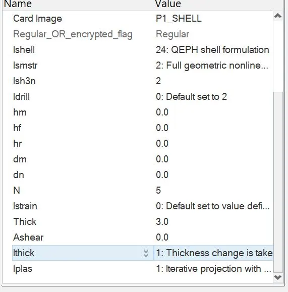
The simulation file is run without making any changes, except optimizing the shell properties.
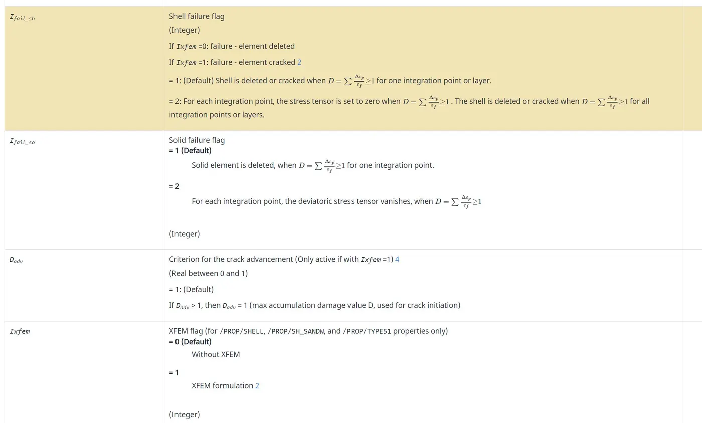
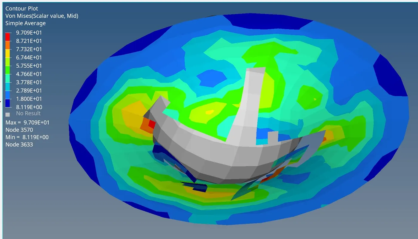
Since IXFEM is OFF, therefore, the failed elements are deleted as mentioned in the documentation
Energy plot:
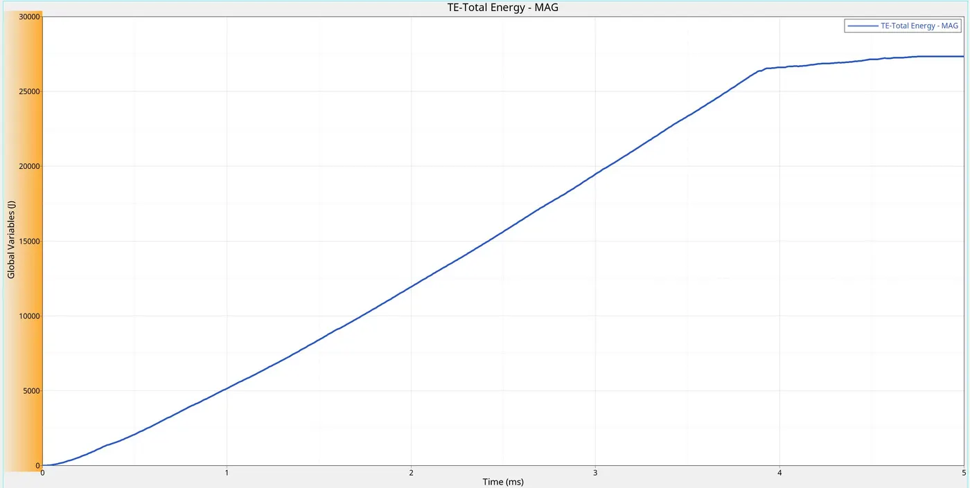
The failure of the element happened when 1 integration point reached Eps_max.
Case 2: Law2_epsmax_crack
The following changes are made
IXFEM formulation is activated, which results in element cracking and not deletion. Since this SHELL Type1, therefore, whole element thickness is considered as 1 layer, hence only one crack appears across the thickness.
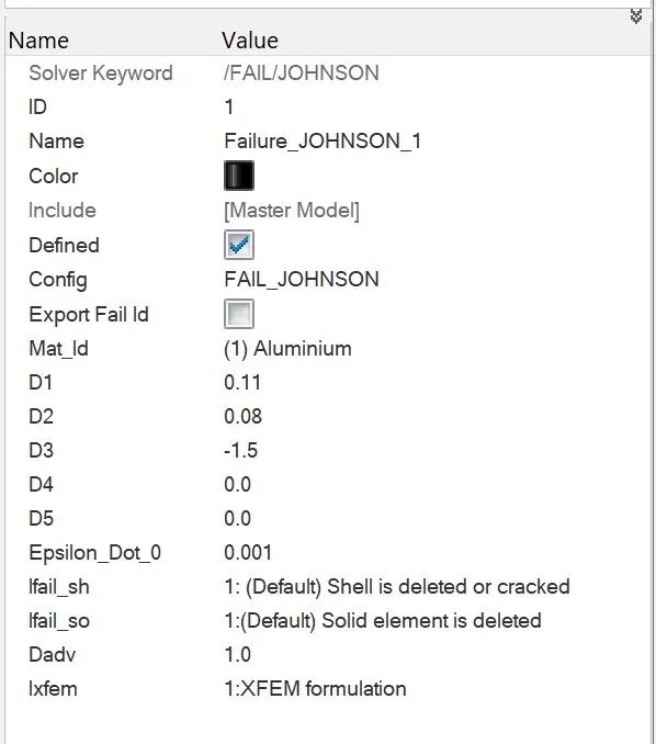
Using the Johnson-Cook failure model /FAIL/JOHNSON along with the Johnson-Cook material model provides more user control of the failure Johnson-Cook failure strain definition:
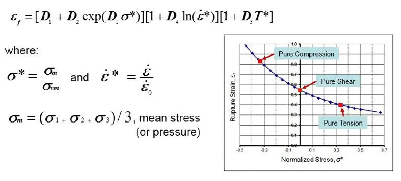
From the "Law2_epsmax_crack_0000.rad"

Failure Strain can be calculated.
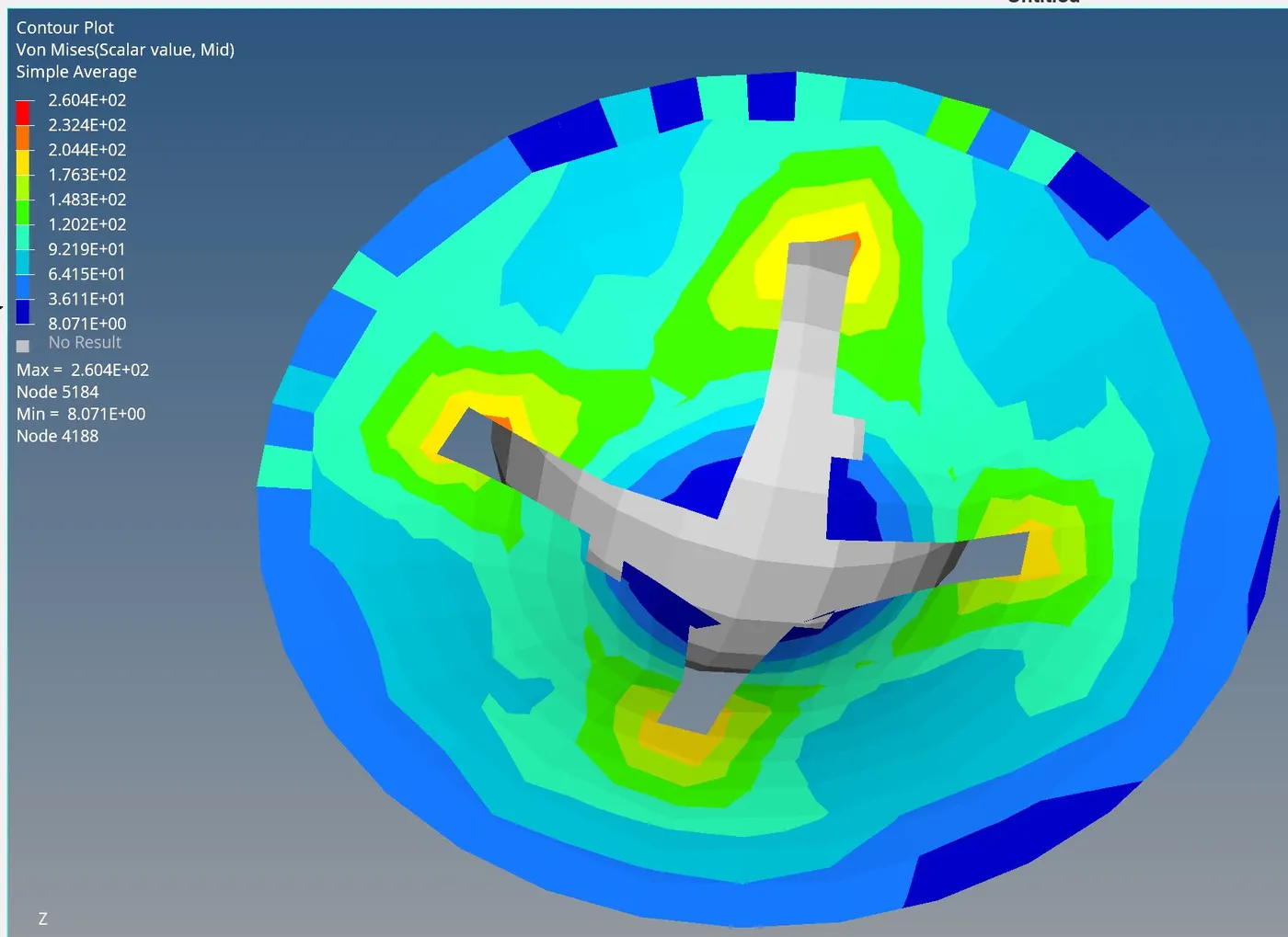
The elements are cracking, and not just simply getting deleted.
Energy plot:
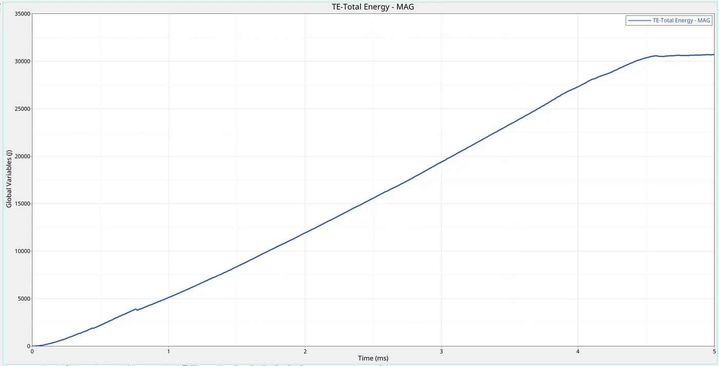
The Energy plot looks no different than the previous plot because the basic formulation remains the same. The failure of the element happened when 1 integration point reached Eps_max.
Case 3: Law2_epsmax_nofail
In this case, the Johnson failure criterion is deleted:
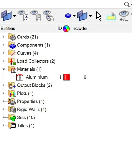
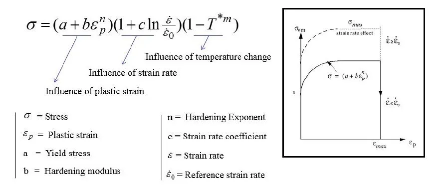
Since there is no Johnson Failure model included in the analysis, the element failure is calculated based on the Johnson-Cook material law model as shown below:
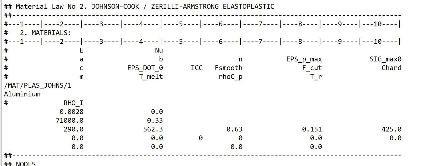
The value of these parameters can be seen in "Law2_epsmax_nofail_0000.rad" as shown:
Energy Plot:
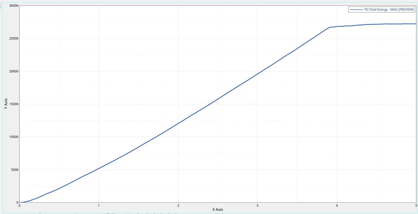
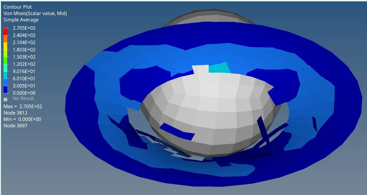
The failure of the element happened when 1 integration point reached Eps_max, and they are deleted.
Case 4: Law2 (EPS_max deleted)
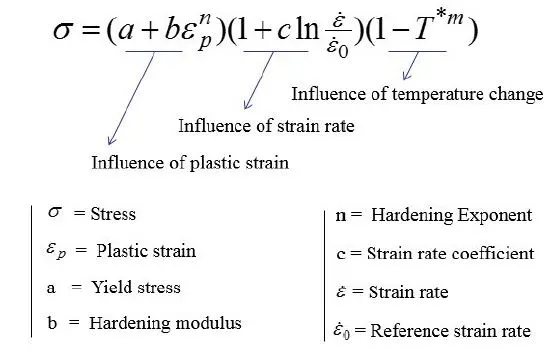
As discussed previously, the Johnson-Cook model is:

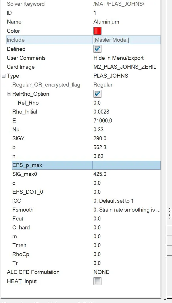
Now, for this case there is no Eps_max defined, therefore no elements are deleted.
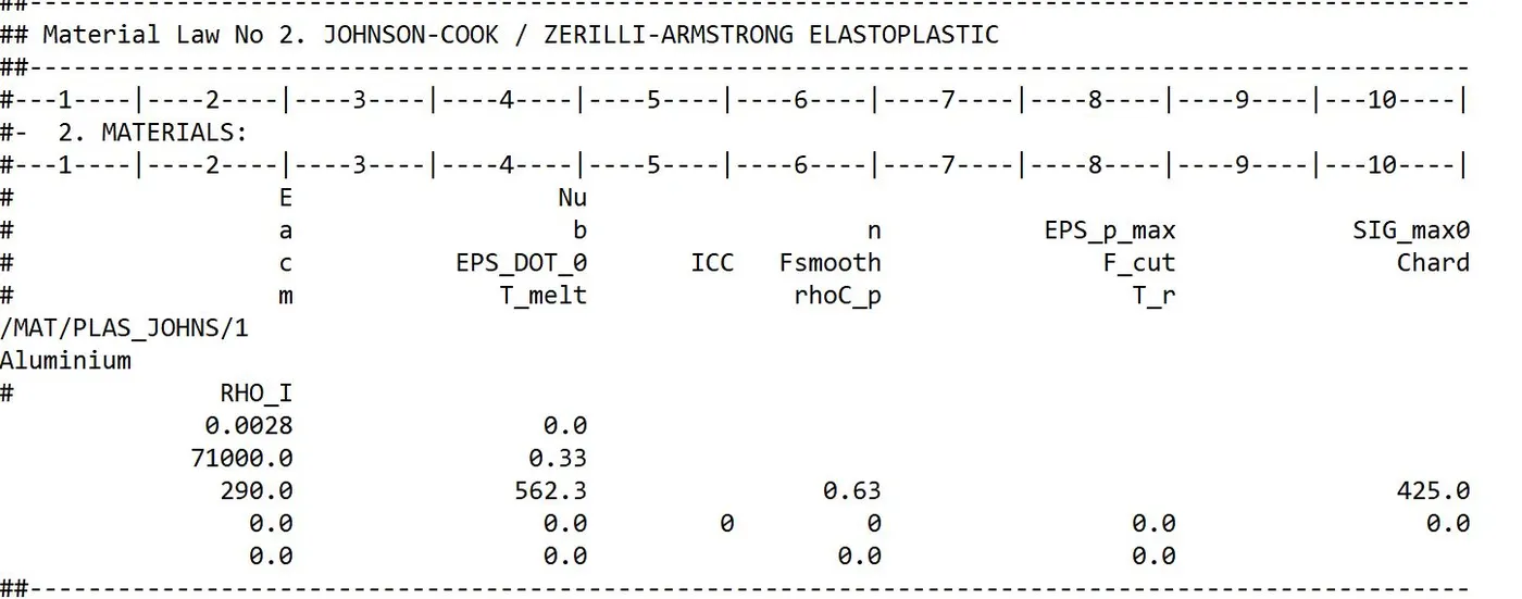
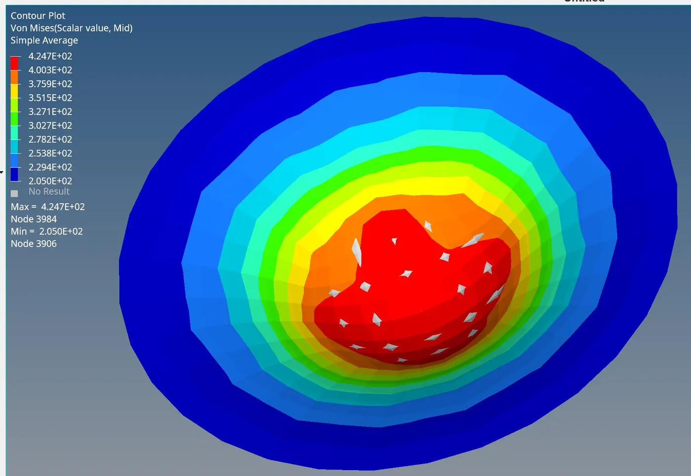
Energy Plot:
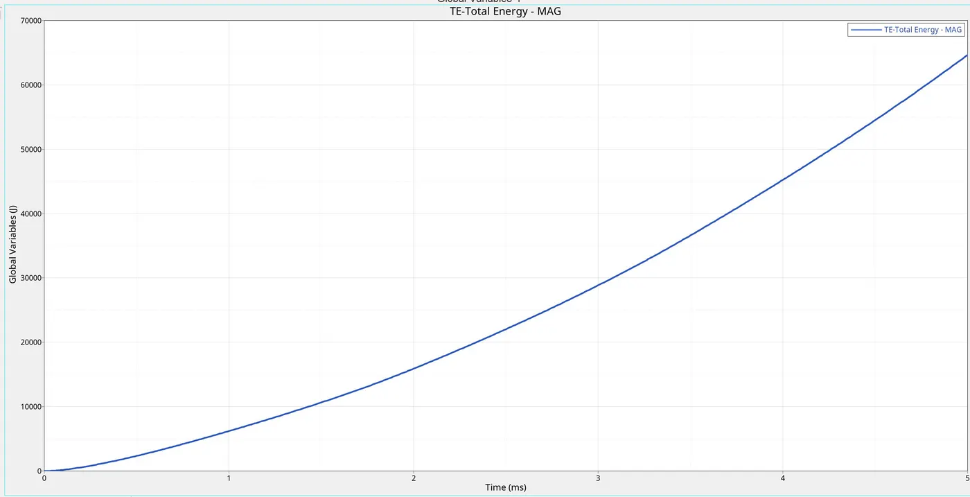
Since no elements are being deleted, the stretching continues, and hence, the energy curve doesn't get flat like the previous cases. The failure occurred after the Yield limit is crossed.
Case 5: Law1
Law 1 is for linear elastic materials only. he material stiffness is determined by only two values: Young’s modulus (E), and Poisson’s ratio (n). The shear modulus (G) can be computed using E and n. Thus, can only be used for parts that are stressed below the yield strength.
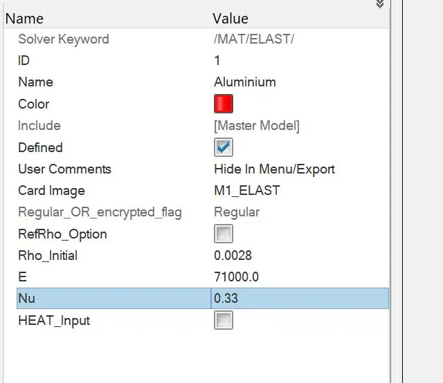
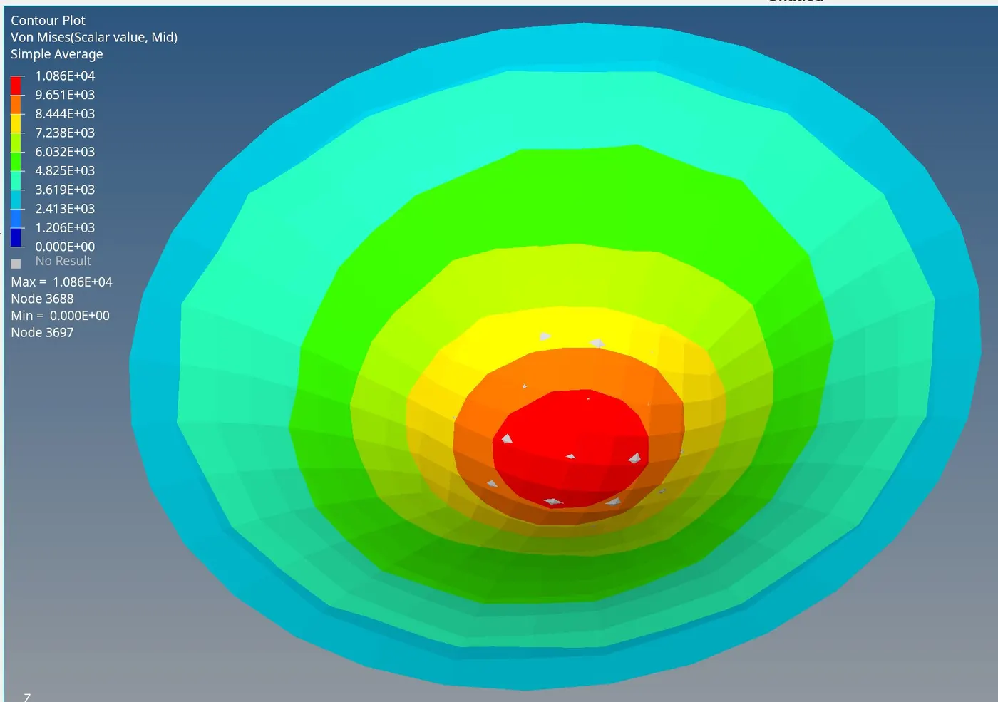
Energy Plot:
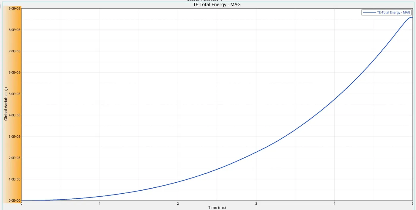
In this case, the failure happened, because the stress crossed the Yield Strength, with no elements being deleted.
Case 6: Law36
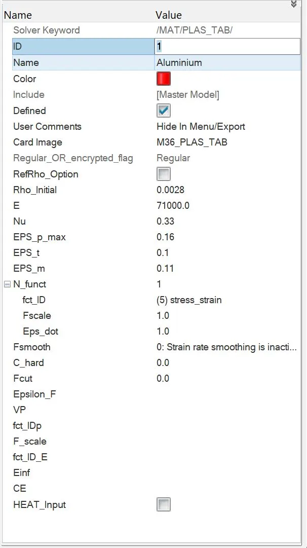
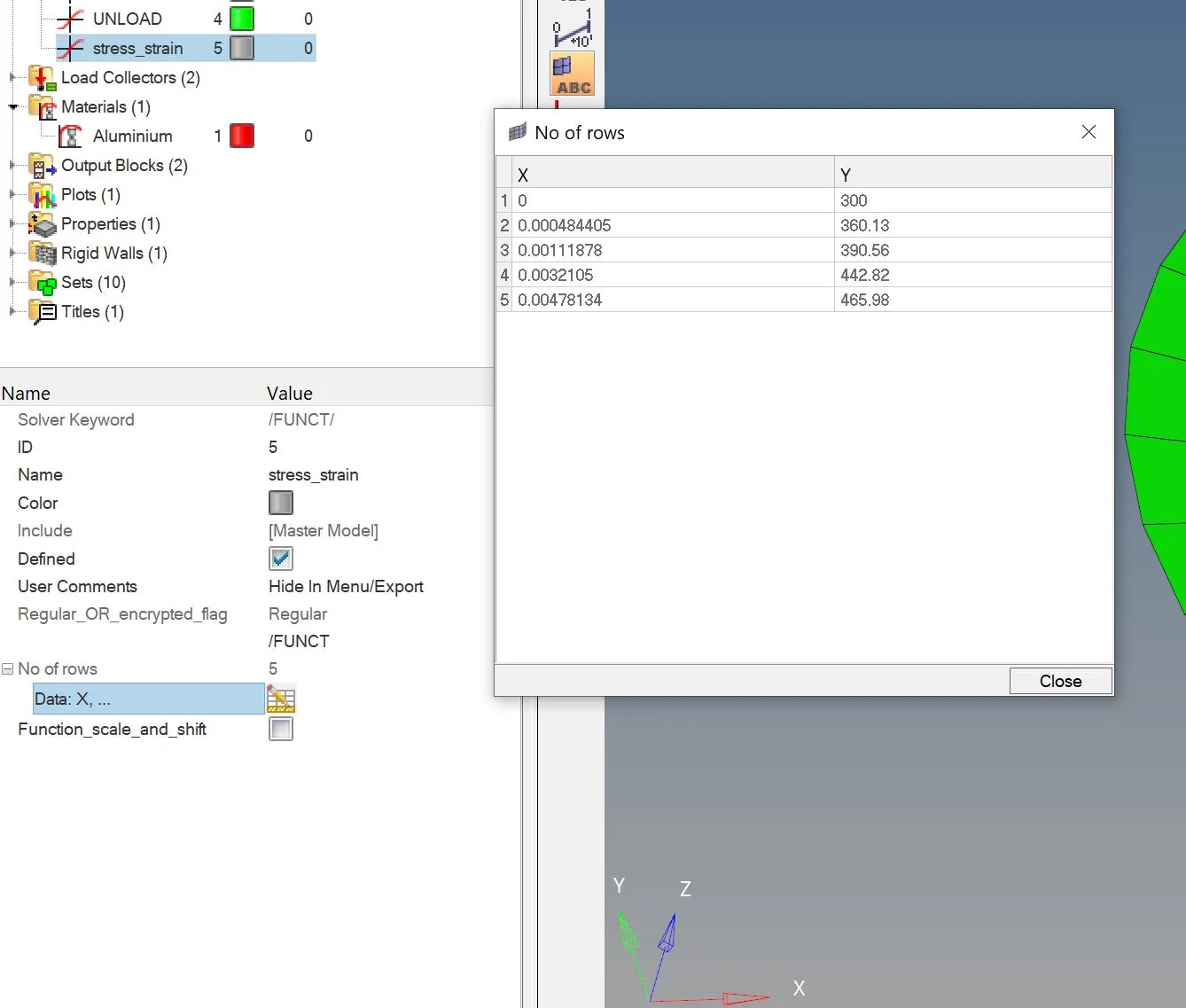
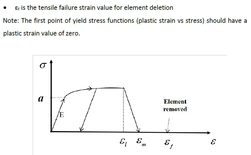
This law models an isotropic elastoplastic material using user-defined functions for the work hardening portion of the stress-strain curve (for example, plastic strain vs. stress) for different strain rates. The property card looked like:
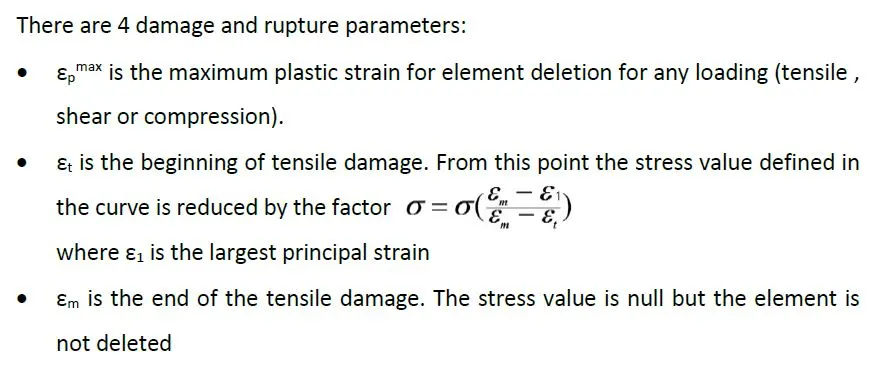
Energy Plot:
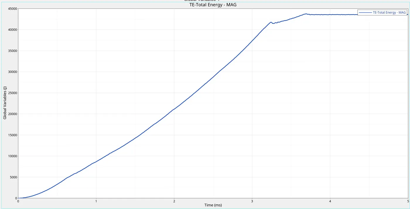
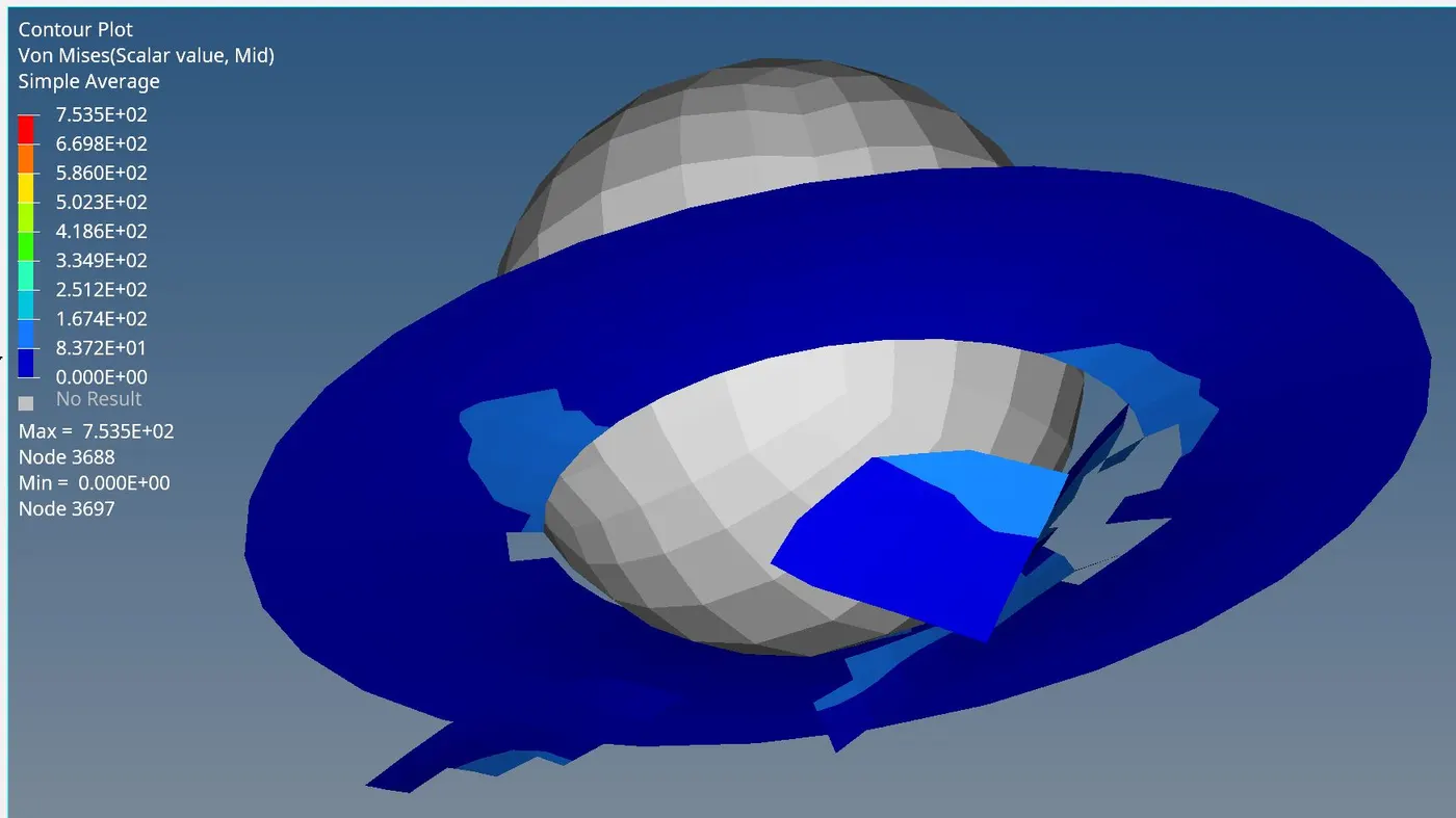
The elements were deleted when the largest Principal Strain reached the Maximum Tensile Failure Strain.
Case 7: Law27
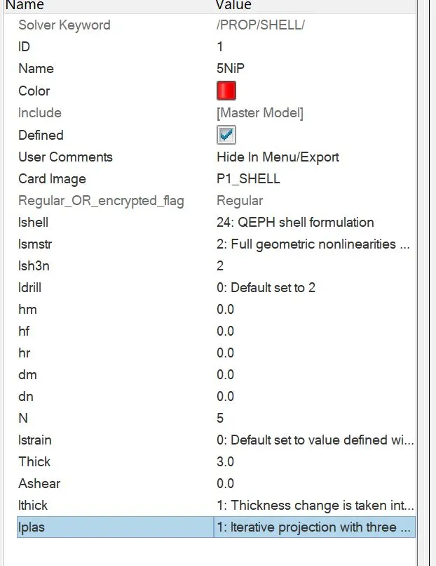
This law combines an isotropic elastoplastic Johnson-Cook material model with an orthotropic brittle failure model. Material damage is accounted for prior to failure. Failure and damage occur only in tension. This law is applicable only for shells.
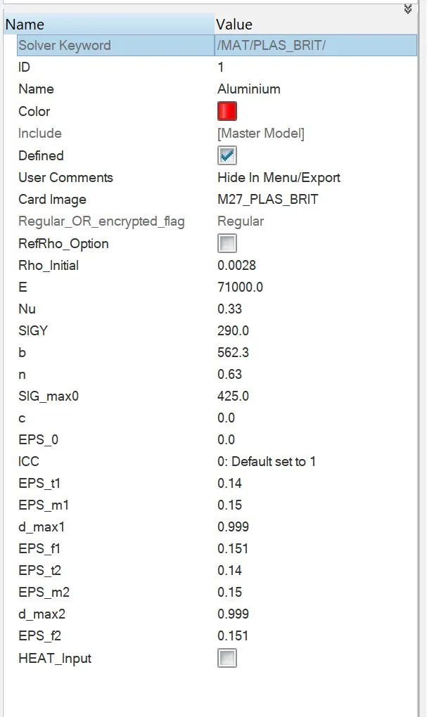
Energy Plot:
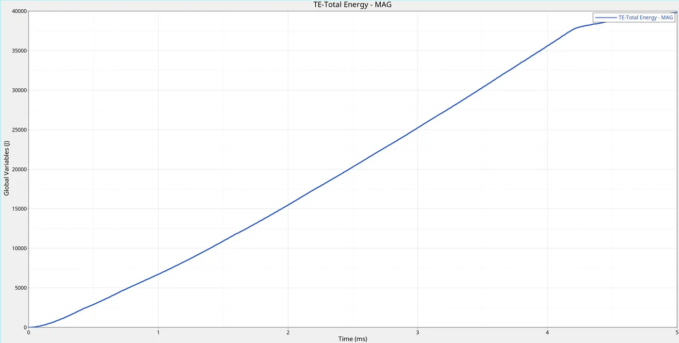
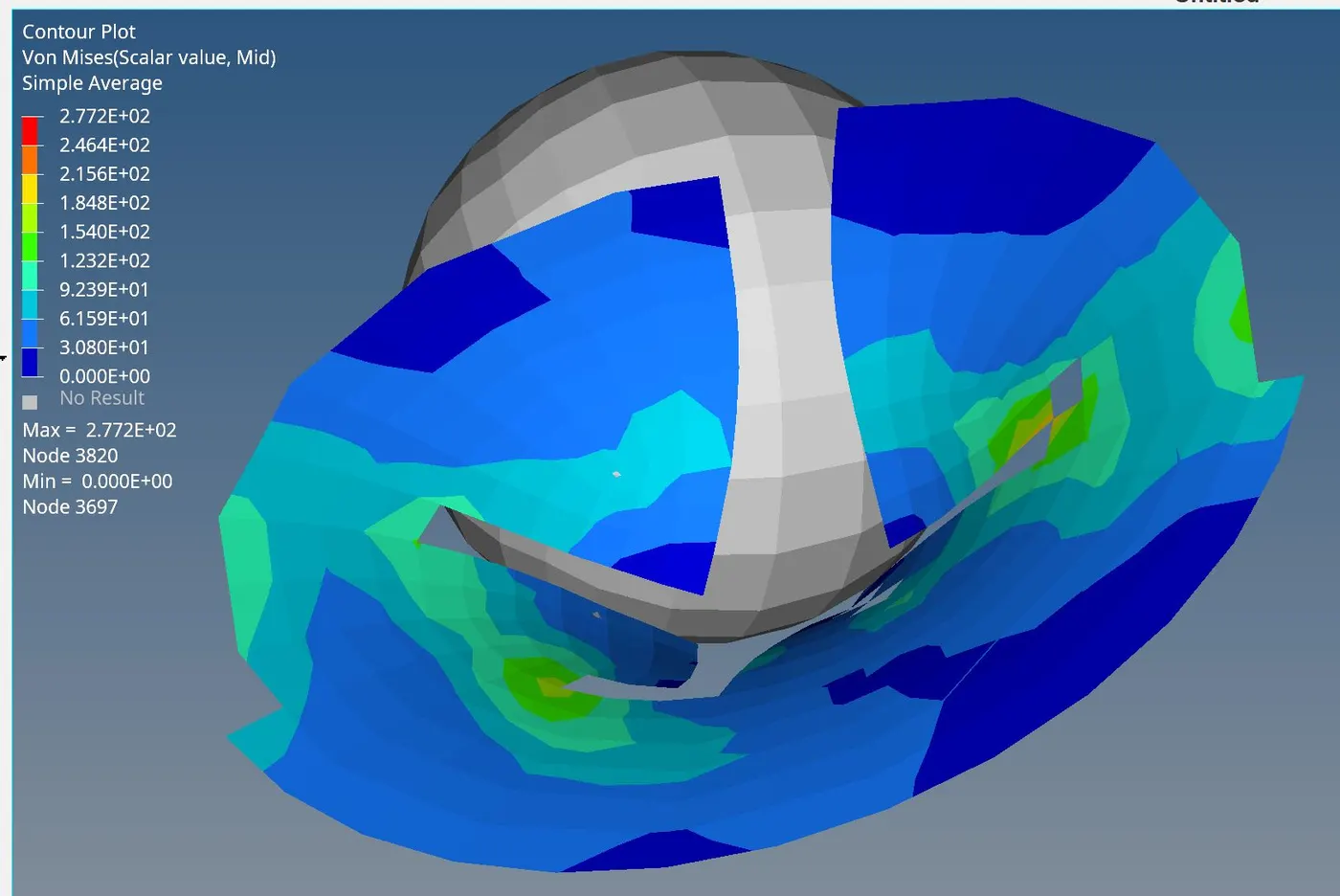
This law is used for brittle materials like glass, hence animation pic depicts here. Elements are being deleted based on Maximum Tensile Strain.
Comparison Table:
| Sr. No. | Case Type | No. of Cycles | Energy Error | Mass Error | Simulation Time |
| 1 | Law2_epsmax_failure | 49479 | 0.2% | 0 | 58.62 s |
| 2 | Law2_epsmax_crack | 49396 | 4.0% | 0 | 58.93 s |
| 3 | Law2_epsmax_nofail | 49404 | 0.8% | 0 | 59.91 s |
| 4 | Law2 | 48736 | 3.0% | 0 | 57.79 s |
| 5 | Law1 | 47968 | 0.3% | 0 | 57.36 s |
| 6 | Law36 | 52203 | 1.5% | 0 | 61.81 s |
| 7 | Law27 | 49355 | 1.1% | 0 | 58.45 s |
Conclusion: After studying all above mentioned was, case 2 seems to represent the on-field condition, because the elements are being cracked, and not deleted.
NOTE: All the cases are attached to the report.