Material cards in Radioss

AIM:

To set up and run the simulation for all the 7 cases in HYPERMESH and compare them to give a proper conclusion.

SOFTWARE:

HYPERWORKS 2020

USER PROFILE:

RADIOSS

PROCEDURE:

CASE 1:

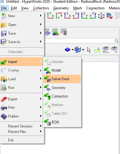
First import the starter file (FAILURE_JOHNSON.0000.rad) in HYPERMESH by going to menu bar > file > import > solver deck. Browse the file from the system and import it.

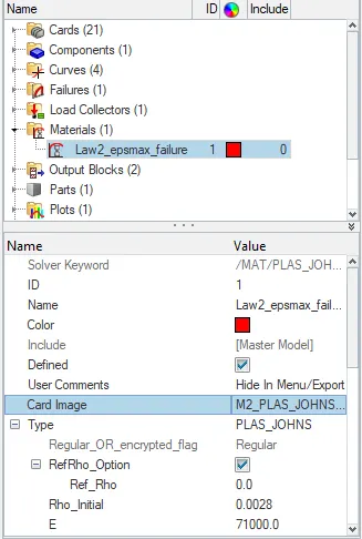
The material card use in this case is M2_PLAS JOHNS. It is also called as Law2 - Johnson cook material card. This is an isotropic elasto-plastic material card.

Once the model is imported, change the material card name to Law2_epsmax_failure and run the simulation as it is. To run the simulation Go to the main menu page > Analysis > Radioss. Click on "save as" to change the file directory to case 1 folder.

Tick the box of include connectors and under options tab, type the value as -nt 4 and click on Radioss to run the simulation.

Once the simulation is started, HYPERMESH will popup a box in which it will show the simulation process.

After the simulation run is completed, a message will show on the popup screen as the job is completed.

All the files which were generated during the simulation run such as .h3d file, T01 file, starter file, engine file, etc will be stored in the input file directory (case 1 folder).

Animation file (.h3d) can be viewed from HyperView.

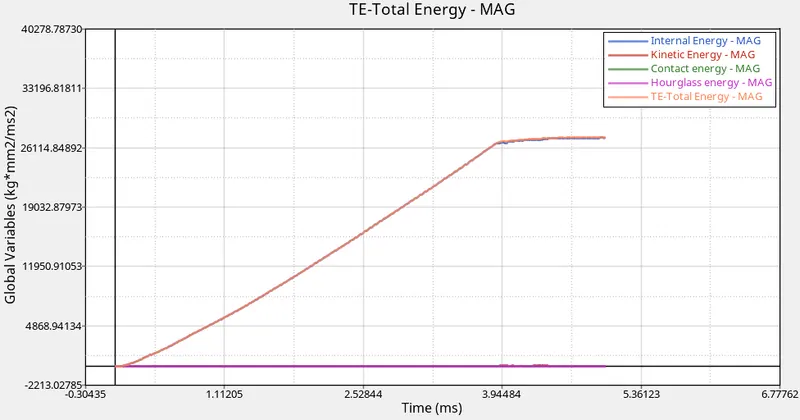
Now plot internal energy, Kinetic energy, contact energy, hourglass energy and total energy of the case 1 simulation in HyperGraph 2D.

The below graph shows the changes in the energies during case 1 simulation run.

CASE 2:

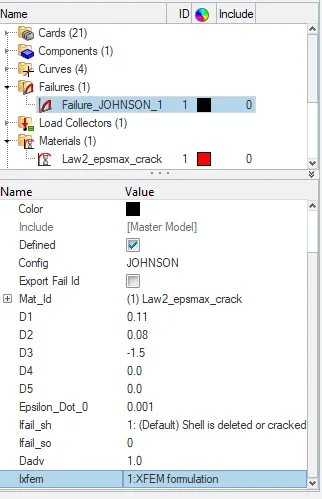
In this case we are using the case 1 starter file and law 2 material card but before running the simulation we are changing the values of the failure card with the below given values.

• Ifail_sh=1- Shell is deleted or cracked for one integration point.
• Dadv=1 - It is a criterion for crack advancement. It will be only active if ixfem is equal to 1.
• ixfem=1 - It actually represents a crack over an element. By defining ixfem=1 it will give room for more realistic behaviour in the system.

But there are some challenges that need to be taken care of if we define ixfem value. They are:

• The material model needs to be very accurate.
• ixfem can be used only for SHELL elements.
• It dissipates little more energy and because of that for very small/local deformations it is a good idea but for large deformations it is not recommended.

After changing the values run the simulation as Law2_epsmax_crack and save it in a separate folder as case 2.

The procedure for running the simulation for this case is the same as mentioned in case 1.

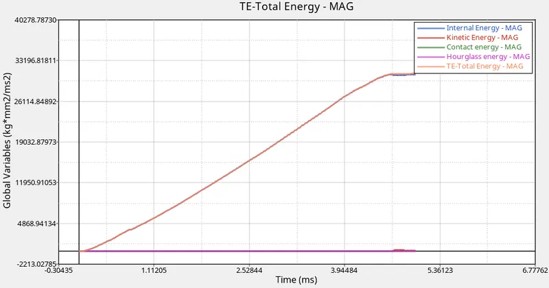
Now plot internal energy, Kinetic energy, contact energy, hourglass energy and total energy of the case 2 simulation in HyperGraph 2D.

The below graph shows changes in the energies during case 2 simulation run.

CASE 3:

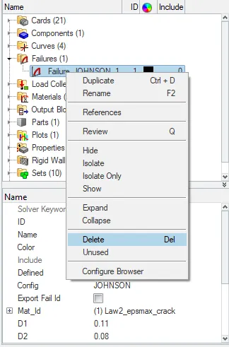
In this case we are using the case 2 starter file and law 2 material card but before running the simulation we are deleting the failure card.

Failure card or Failures:

Failure of the element happens when 1 integration point reaches EPS_p_max value. The failing of elements in a regular/non-regular manner depends upon the failures. By changing or editing the failure card the elements failing in a non-regular manner during simulation can be avoided.

After deleting the failures run the simulation as Law2_epsmax_nofail and save it in a separate folder as case 3.

The procedure for running the simulation for this case is the same as mentioned in case 1.

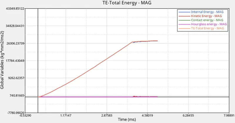
Now plot internal energy, Kinetic energy, contact energy, hourglass energy and total energy of the case 3 simulation in HyperGraph 2D.

The below graph shows changes in the energies during case 3 simulation run.

CASE 4:

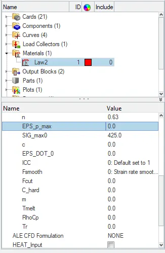
In this case we are using the case 3 starter file and law 2 material card but here we are modifying or deleting the EPS_p_max value. That means in this case the EPS_p_max value will be equal to zero.

EPS_p_max:

• EPS_p_max is plastic failure strain for tension, compression or shear.
• Consider EPS_p_max value as 0.40. That means the material is going to fail at 40% plastic strain.
• Once the material reaches at 40% plastic strain the fail element will either break into pieces (if ixfem=0) or it may get deleted (if ixfem=1) from the system.

After deleting the EPS_p_max value run the simulation as Law2 and save it in a separate folder as case 4.

The procedure for running the simulation for this case is same as mentioned in the case 1.

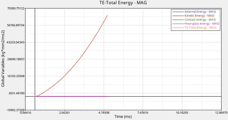
Now plot internal energy, Kinetic energy, contact energy, hourglass energy and total energy of the case 4 simulation in HyperGraph 2D.

The below graph show changes in the energies during case 4 simulation run.

Case 5:

In this case we are converting the above material model (Law2 material model which was used till case 4) to Law1 elastic material with same density, young's modulus and poisson's ratio.

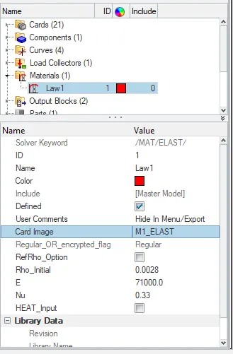
Law1: M1_Elast:

To define elasticity we need to define only three points i.e, density of the material, young's modulus (E) and poisson's ratio (Nu).

Using these 3 values we can calculate almost each and every other detail of the material.

Below mentioned values were used in this case to run the simulation.

• Density = 0.0028
• Young's modulus (E) = 71000
• Poisson's ratio (Nu) = 0.33

After applying the above values run the simulation as Law1 and save it in a separate folder as case 5.

The procedure for running the simulation for this case is the same as mentioned in case 1.

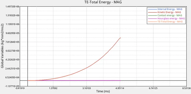
Now plot internal energy, Kinetic energy, contact energy, hourglass energy and total energy of the case 5 simulation in HyperGraph 2D.

The below graph shows changes in the energies during case 5 simulation run.

CASE 6:

In this case we are using the case 5 starter file and law 36 material card. Law 36 PLAS_TAB material card is also called as Elastic plastic piece wise linear material card.

Law36: M36_PLAS_TAB:

Elastic plastic piece wise linear material card is the most commonly used material model in the industries. This is because in the real time situations we are not always able to determine the proper yield stress number, failure parameters, failure properties of the plastic region behaviour.

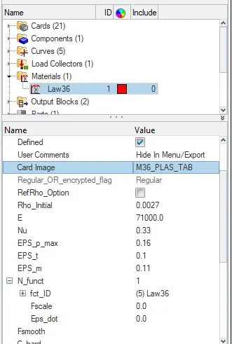
The values for the law 36 material card is given below.

• Density = 0.0027
• Young's modulus (E) = 71000
• Poisson's ratio (Nu) = 0.33
• EPS_p_max = 0.16
• EPS_t = 0.1
• EPS_m= 0.11
• N_funct= 1

EPS_t - Tensile failure plastic strain. It is the point where the stress starts coming down to zero.

EPS_m - Stress is equal to zero.

N_funct - Number of functions

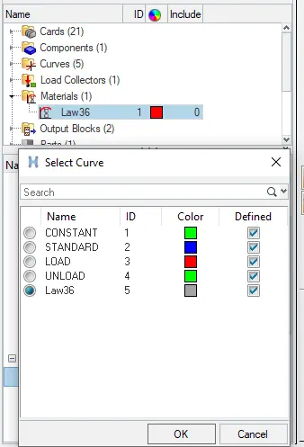
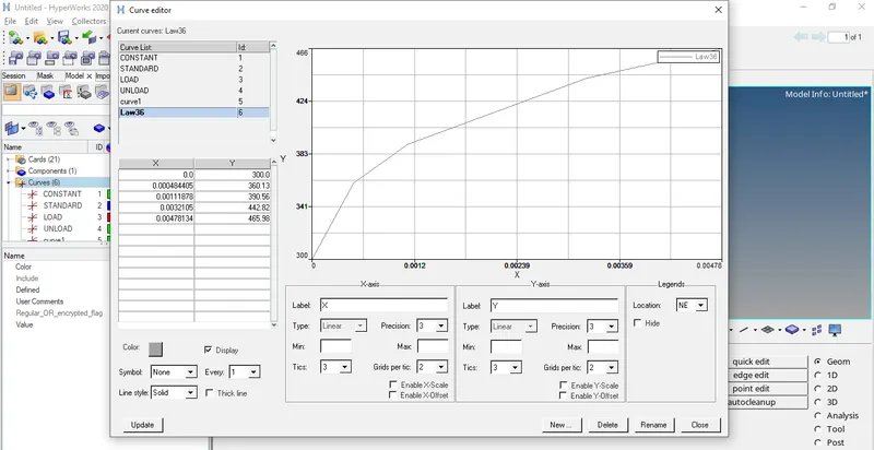
In law36 we put the data curve manually. Because of the rapid movement in the material the strain rates are very rapid that's why we cannot predict at what strain rates the deformation is happening at various components thus in this material card it is better to test the material at different strain rates and put all this curves under user defined functions while creating the PLAS_TAB card as shown in the below figure.

After applying the above values run the simulation as Law36 and save it in a separate folder as case 6.

The procedure for running the simulation for this case is the same as mentioned in case 1.

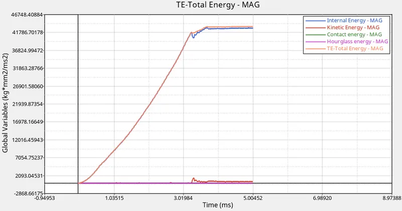
Now plot internal energy, Kinetic energy, contact energy, hourglass energy and total energy of the case 6 simulation in HyperGraph 2D.

The below graph shows changes in the energies during case 6 simulation run.

CASE 7:

In this case we are first importing a new starter file i.e Law27_0000.rad file. The material card used in this case is M27_PLAS_BRIT. This card is an isotropic elasto-plastic material with brittle failure.

Law27: M27_PLAS_BRIT:

The PLAS_BRIT material card is specially used for brittle materials. This law combines an isotropic elasto-plastic Johnson-cook material model (Law2) with an orthotropic brittle failure model.

Before running the simulation change the shell properties to recommended shell properties as shown in the below figure.

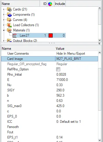
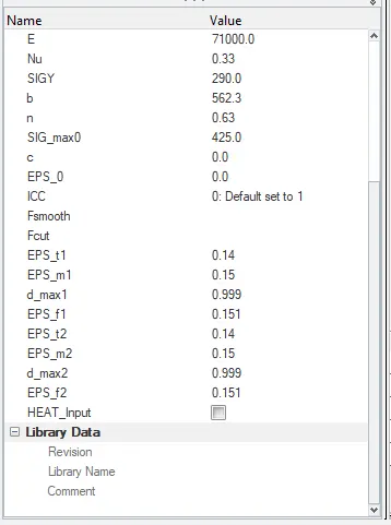
• dmax - It will accelerate the failure of the element.
• EPS_f - Maximum tensile strain for element deletion (element removed from the system).

After applying the above values run the simulation as Law27 and save it in a separate folder as case 7.

The procedure for running the simulation for this case is the same as mentioned in case 1.

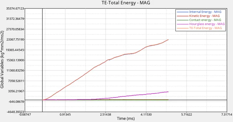
Now plot internal energy, Kinetic energy, contact energy, hourglass energy and total energy of the case 7 simulation in HyperGraph 2D.

The below graph shows changes in the energies during case 7 simulation run.

Comparison of case 1 and case 2:

Animation (.h3d) of case 1 vs case2:

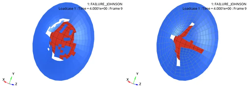
The elements in case 1 are getting deleted from the system. As we have run the simulation as it is in case 1, the ixfem value was kept to zero by default. Thus the elements will get deleted if the ixfem value is kept to zero.

What is ixfem?

The ixfem value can be found under the failures. It will help us to decide how we want to fail a particular element. If we keep the ixfem value to '0' it will simply delete the whole element from the simulation (case 1).

If we keep the ixfem value to '1' then it will try to break the element the way it should have cracked under the given force or loading conditions (case 2).

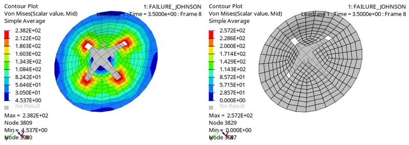
As we can see from the above figures the elements in case 1 (left) are getting deleted from the system in a non-regular manner while in case 2 (right) the elements are getting cracked in a regular manner and a proper whole is being generated.

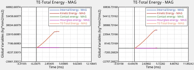
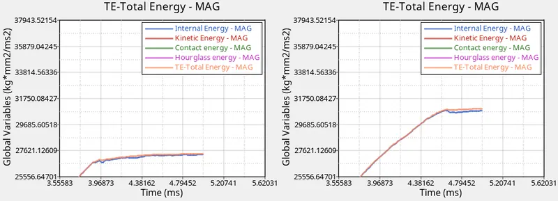
From the above graphs of case 1 and case 2 it can be observed that the internal energy and total energy is getting distorted after a certain point. This is because the elements are getting deleted from the system.

when the elements are getting deleted there will be fluctuations in the energy curve. since we have define ixfem value in case 2 the elements are getting deleted in a regular manner.

Deletion of elements in case 1 is earlier as compared to case 2 which can be observed from the above animation images and graphs.

Comparison of case 3 and case 4:

Animation (.h3d) of case 3 vs case4:

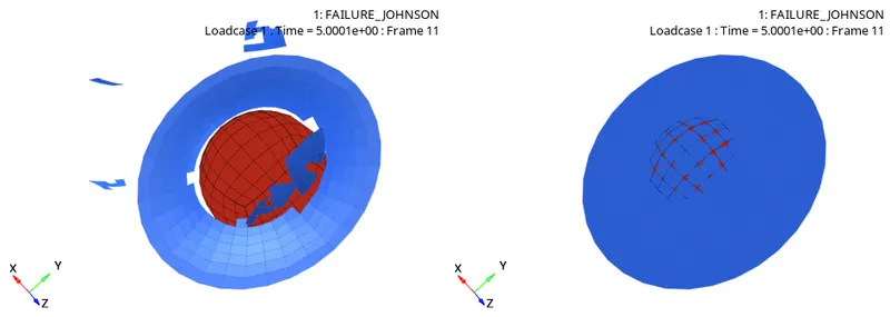
In the case 3 we can see that a hole is being generated but the deletion of the element is not in a regular manner. This is because we have deleted the failure in the above cases.

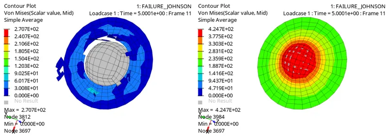
while in case 4 EPS_p_max was kept zero which results in the elements going to infinite strain.

Since we have defined the SIG_max0: 425 in case 4, you can notice that the stress has not exceeded that value. If the stress has been exceeded further the elements will be deleted from the system.

In case 3 EPS_p_max=0.15 that means the element is going to fail at 15% plastic strain after which the element will be deleted from the system

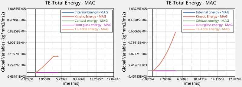
The elements are getting deleted at 15% plastic strain which can be observed from the change in internal and total energies in case 3. Since we have defined the EPS_p_max value, less stress has been generated in the system.

while in case 4 since there is no deletion of elements we can notice that there are no changes in internal and total energies but more stress has been generated in the system.

Comparison of case 5 and case 6:

Animation (.h3d) of case 5 vs case6:

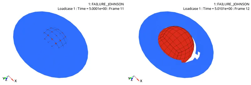
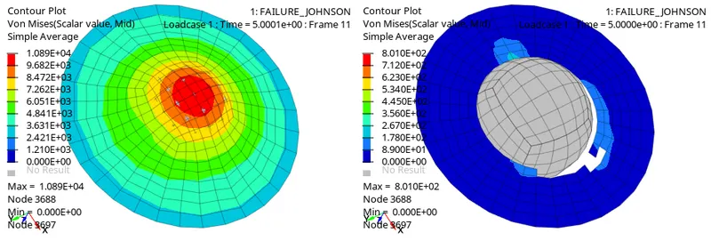
In case 5 we have used Law1 elastic material. In elasticity whatever deformation it creates the system will comeback to zero stress once the force is removed.

• Law1 elastic material should not be used for parts undergoing large deformation.
• Elastic material is not recommended for crash analysis.

In case 6 we have used Law36 PLAS_TAB material. From the above animations we can see a proper hole is generated in the case 6 PLAS_TAB at very lower stress.

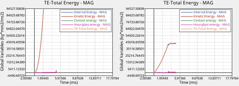
Because of the high stress developed in case 5 we can observe that the internal and total energies in the graph is very high compared to the case 6 graph.

Law36 PLAS_TAB can be used for all types of elements like brick elements, shell elements etc.

The failure is easy to manage in this law.

Comparison of Law2 and Law27 (case 7) material card:

In case 7 we have used the Law27 PLAS_BRIT material card. This material card is specially used for brittle materials. In both the cases no failure was used.

Animation of PLAS_JOHN material card against PLAS_BRIT material card:

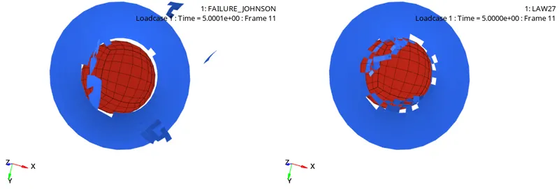
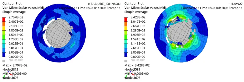
From the animation it can be observed that a proper hole is generated with low stress developed in the law2 material card while in law27 the element deletion is in a non-regular manner and more stress being generated in the system.

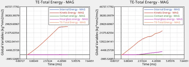
Change in internal,total and hourglass energies can be observed from the case 7 graph. This is due to the following reasons:

• Plastic region is very narrow in this material card.
• They are prone to failure much quicker.
• Material damage is accounted for prior to failure.
• failure and damage occur only in tension.

PLAS_BRIT material card is better than a PLAS_JOHN material card in case of brittle materials. It is useful for modeling brittle failure of glass.

The change in internal energy and total energy in law2 material card is due to the element deletion. When the elements are getting deleted from the system there will be few fluctuations in the energy curves which can be seen in the law2 graph.

Based on all the results, the Law1 elastic material can represent the on field scenario. For example:

Rubber materials, both natural and synthetic are examples of elastic materials. Elastic materials are materials which show high elasticity i.e, which can be stretched several times its original length and upon releasing of the stress, it returns back to its original shape and dimensions.

Total number of cycles, Energy error, mass error and simulation time:

Depending on the material model and failure criteria the number of cycles, energy error and mass error will differ. All the values for the below mentioned cases are given in the following table.

Cases	Total number of cycles	Energy error	Mass error	Simulation time (in seconds)
Case 1	49380	0.8%	0.2721E+05	60.04
Case 2	49217	4.1%	0.2980E+05	65.55
Case 3	49408	0.8%	0.2736E+05	59.85
Case 4	48737	3.0%	0.6298E+05	59.04
Case 5	47969	1.3%	0.8568E+06	59.97
Case 6	53155	-1.3%	0.4432E+05	65.01
Case 7	41113	-7.1%	0.2547E+05	49.34

RESULT:

The simulation results for all the cases have been successfully obtained and the comparison for the same is mentioned in the above report.

CONCLUSION:

Out of all the four law material cards (i.e Law 1,2,27,36) which were used in the above 7 cases, the Law36 PLAS_TAB or Elastic plastic piece wise linear material card is the most widely used material card in the industries because the failure can easily be managed and it can be used for all types of elements. Thus this material card is recommended to use when compared to the above mentioned material cards.