Assignment 3-2D Element Formulation Challenge

Assignment 3

Aim

To compare the results of simulation before and after property assignment for the given crash beam file

Procedure

• Import the .rad file to hypermesh

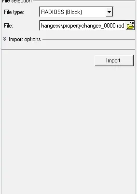
Figure 1

• Change the tstart to 25 ms in Eng_Anim_Dt and Tstop in Eng_Run to 55ms

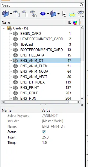
Figure 2

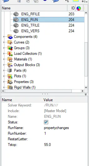
Figure 3

• After making the changes,export the file to a separate folder.
  It is better to export to a new folder as after running the simulation, radios generates several files which can confuse the user.

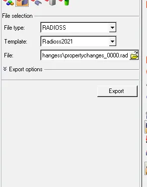
Figure 4

• Now, we can run the simulation with the default property settings using Analysis->Radioss

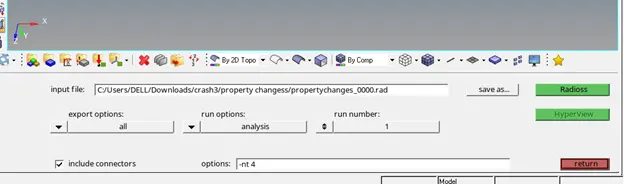
Figure 5

• Select the appropriate input file and start radios and wait for the solver to finish.
• After it has finished,radios will generate output files,animation files to be viewed using hypergraph/hyperview respectively.

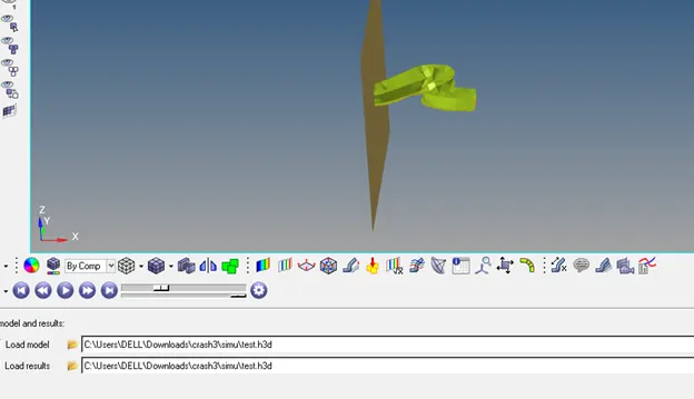
Figure 6

• The .0001 output files are important for energy and mass error checks
• The recommended property values for crash applications are given in figure 7

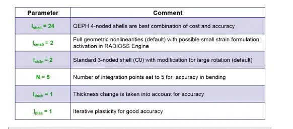
Figure 7

• These values can be modified in the properties tab.

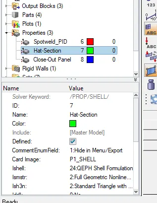
Figure 8

• Make the appropriate changes as shown in figure 7 and export this file to a different folder.
• Now run this file in analysis->radioss and wait for the solver to finish.
• Compare and contrast the differences between the 2 different simulations.

Comparison

• The energy error must be negative and decreasing ,except for the first cycles or in spring back stage, the error must be below 15% at the end of the model (5% or less for a good model)
• In the case of QEPH shell formulation or fully integrated elements, the energy can be slightly positive as there is no hourglass formation and the result is much more accurate.An error of 1-2% is considered acceptable,anymore indicates that energy has been created and there is a model issue.
• The energy and mass error checks can be done by opening the 0001.out files in a text editor.

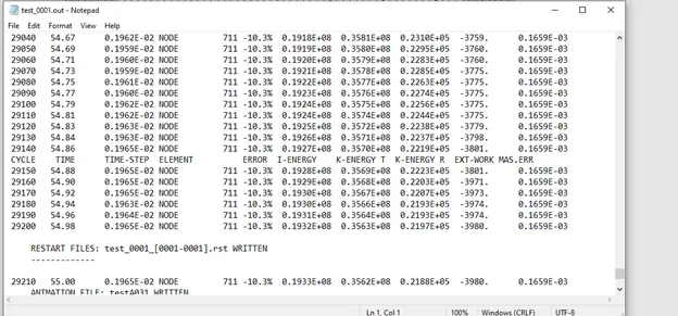
Figure 9

• It is seen that running the simulation with default values for properties gives us an energy error % of -10.3% and a mass error of 0.1659E-03 which is considered acceptable for further calculations
• In the case of the second simulation, the energy % is -0.1% and mass error is 0.1659E-03 which is excellent and can be processed for further calculations.

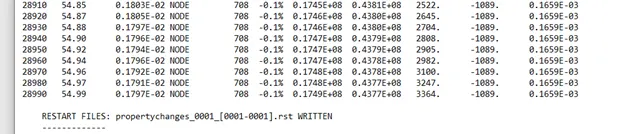
Figure 10

• This significant difference in error % is due to the property changes which give a much better result.
• We can view the animated simulation in hyperview.
• The simulations with and without property changes can be seen in figure 11 and 12.

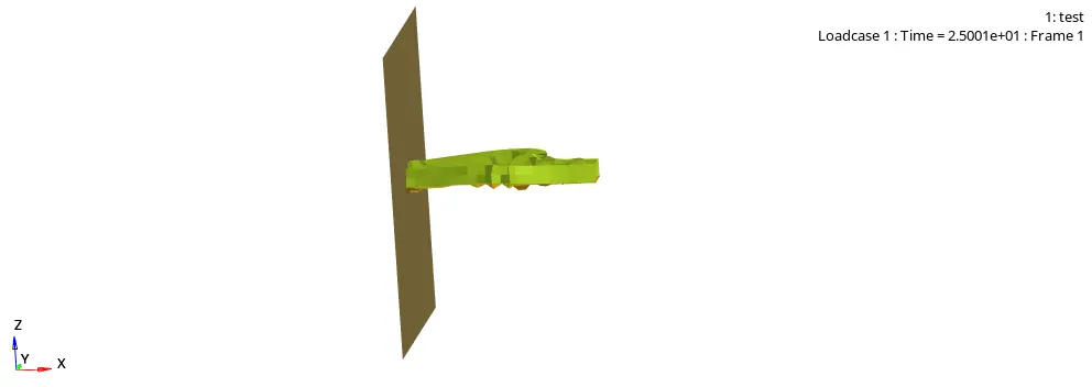
Figure 11

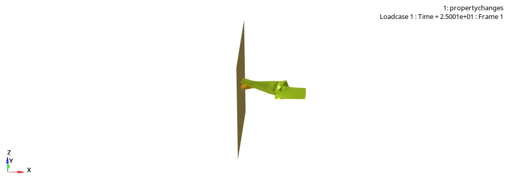
Figure 12

• It can be seen that the deformation observed in figure12 is more realistic compared to that in figure 11
• Now , we go to hypergraph 2D and plot various graphs such as internal energy,contact energy,hourglass energy , rigid wall forces and total energy.

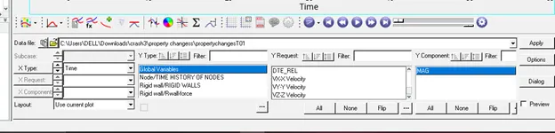
Figure 13

 

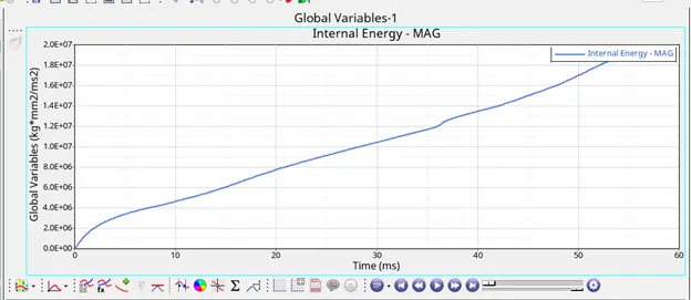
Figure 14 simulation 1

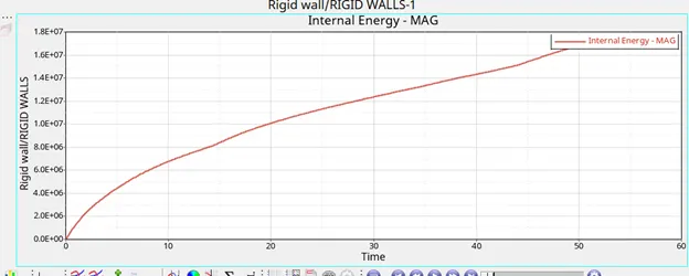
Figure 15 simulation 2

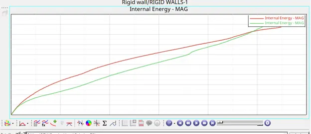
Figure 16

• It can be observed that in the case of the first simulation,the graph is more linear.
• Contact energy for the 2 simulations can be seen in figure 17 and figure 18.

 

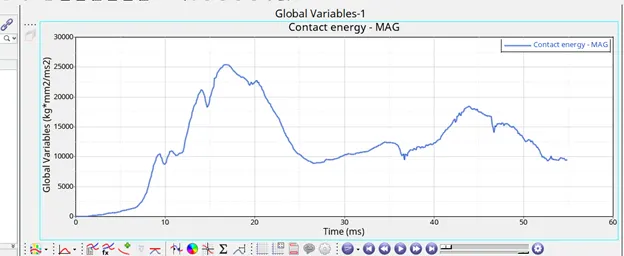
Figure 17 Simu 1

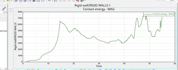
Figure 18 Simu 2

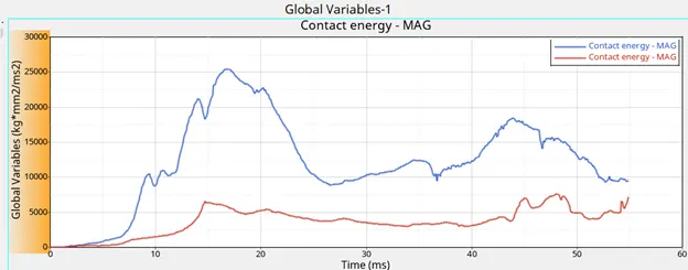
Figure 19

• In both cases,there is a spike at around 15ms that occurs due to the buckling of the component.It is represented more accurately in the second simulations.
• Hourglass energy graphs are depicted in figure 20 and figure 21.
  

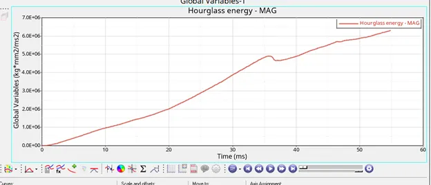
Figure 20 Simu 1

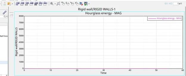
Figure 21 Simu 2

• It can be observed that there is no hourglass energy formation in simulation 2, this is due to the stability provided by QEPH elements
• When elements in a model deform but the strain energy is not computed for that deformation,then it results in hourglass formation.
• The physical stabilization provided by QEPH elements significantly control hourglass formation
• Other methods to solve hourglass formation is to add stiffness to the reduced integration element,an appropriate damping force or by increasing mesh refinement in the area.
• The total energy curves for both simulations are plotted in figure 22 and figure 23.

 

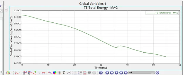
Figure 22

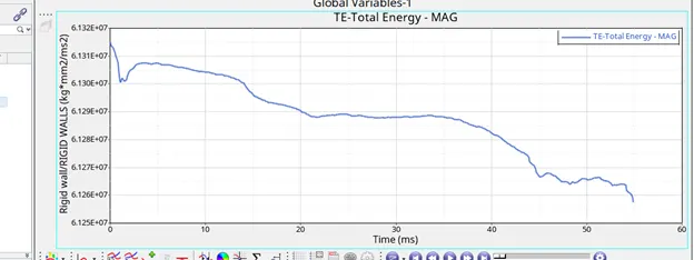
Figure 23

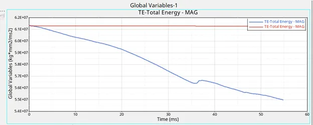
Figure 24

• On comparing the 2 curves,it can be seen that the total energy is approximately constant in simulation 2 while in simulation 1 it decreases linearly
• The rigid Wall forces are plotted accordingly.

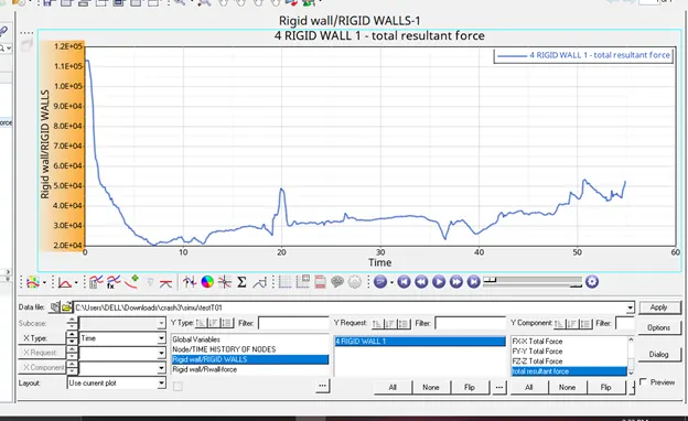
Figure 25

 

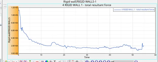
Figure 26

• It can be seen in both cases that the initial force is large due to the first impact.
• The force decreases due to the deformation of the body and a conversion of the force into frictional force.

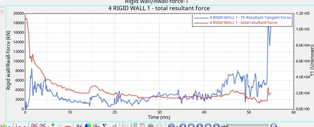
Figure 27

Learning Outcomes

• Property Assignment to elements
• Hourglass formation and how to avoid it
• Using Radioss solver in hypermesh
• Analysing the results of the solver and evaluating it
• Using hyperview and hypergraph to visualize the results.

Result

The given crash beam file was solved with and without property assignment.

The results of the 2 simulations were then compared accordingly.

It can be concluded that proper property assignment can maximize solver time and accuracy of the results according to the engineers needs.