2D Element Formulation in Radioss

Objective: Comparision of 2D shell element formulations with beam crash example.

Procedure:

• Import the 0000.rad file (started file) into hypermesh.

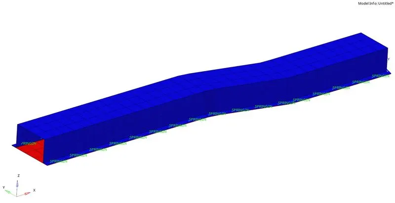
Fig 1: Geometry information contained within the starter file.

Case 1: Default settings.

• Change the simulation time from 60ms to 55 ms in the "ENG_RUN" card.

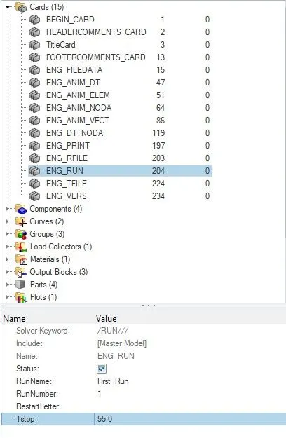
Fig 2: Simulation time is set in the Tstop row.

• For obtaining 25 animation steps for the results, the Tfreq value is changed to 0.9166 (total simulation time/number of animation steps required) in the "ENG_ANIM_DT" card.

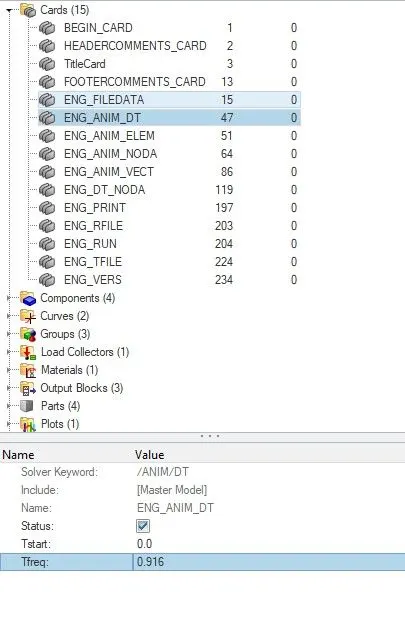
Fig 3: Required number of animation steps are set.

• Rest all card values are left as it is.
• Now we can proceed to run our simulation. Navigate to the analysis tab and choose the radioss option.
• Input file option will be available to save the starter and engine file in the desired location.
• In the options bar, "-nt 6" is entered, which denotes parallel processing for the simulation.

Fig 4: Options in the radioss tab, where the file location and other options for running the simulation are chosen.

• Once all the options are selected correctly, click on the radioss button to run the simulation.
• A separate window pops up and shows the calculation going on, and it might take up to few seconds to minutes based on the complexity of the solution.

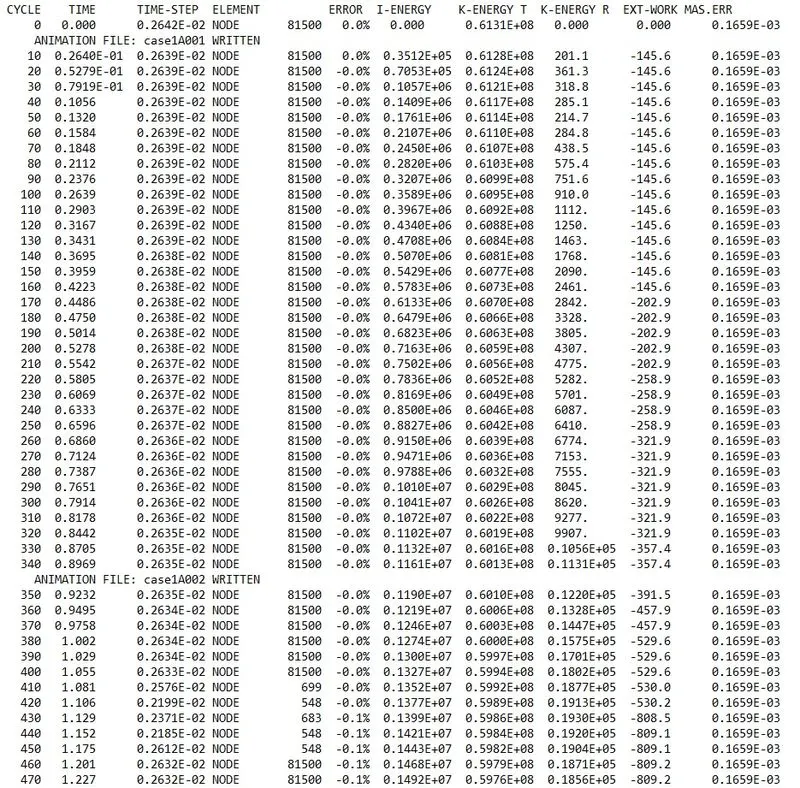
Fig 5: 0001.out files contains the solution information.

• We can check for the energy and mass error from the engine output file whether it lies within the permissible limit or not.
• The energy error starts from -0 to -10%, and the mass error is 0.1659E-03. Both are in the acceptable range, and we can proceed with the post-processing of our results.

Results:

• For post-processing the results Hyperview and hypergraph are used.
• When hyperview is open, we need to load the model and results file of our simulation.

Fig 6: Result file is browsed.

• The h3d file is feed in both columns.

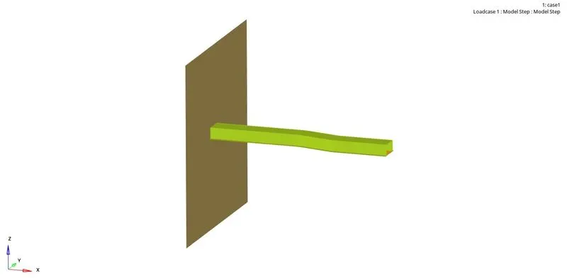
Fig 7: Loaded result file.

• To visualize the contours, we navigate to the contour option, in which we have multiple options to see the results.

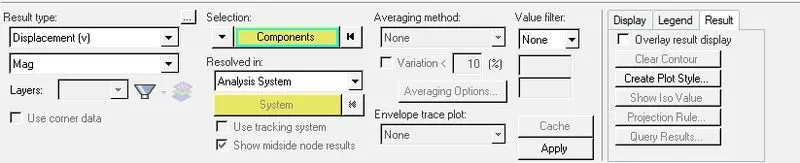
Fig 8: Contour options.

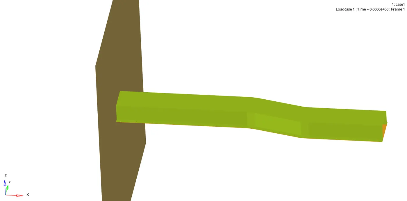
• The above animation represents the crash of rail to the rigid wall.

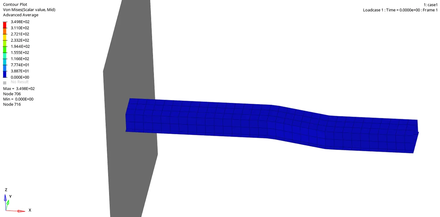
• The above animation represents the von mises stresses generated in the rail.

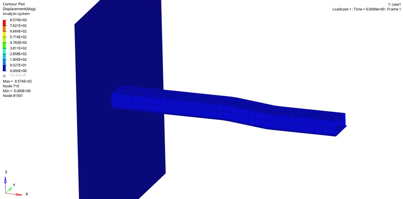
• The above animation represents the displacement produced in the rail.

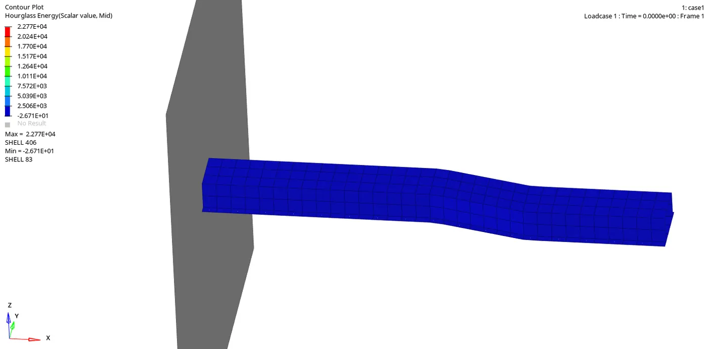
• The above animation shows the hourglass energy being produced in a few of the elements.

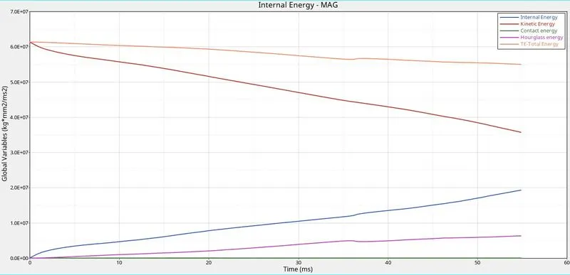
• The above plot shows the Total energy, Kinetic energy, Internal energy, hourglass energy, and contact energy.
• The total energy is the summation of an internal, kinetic, hourglass, and contact energy.
• Kinetic energy initially is higher because the system moves with a certain velocity and is hitting the rigid wall, as the model crashes the wall and finally comes to rest, so the kinetic energy decreases as the simulation goes on.
• Internal energy is the sum of kinetic and potential energy in a system.
• Contact energy is formed because the rail comes in contact with the rigid wall, and the connection between them is the same throughout the simulation.

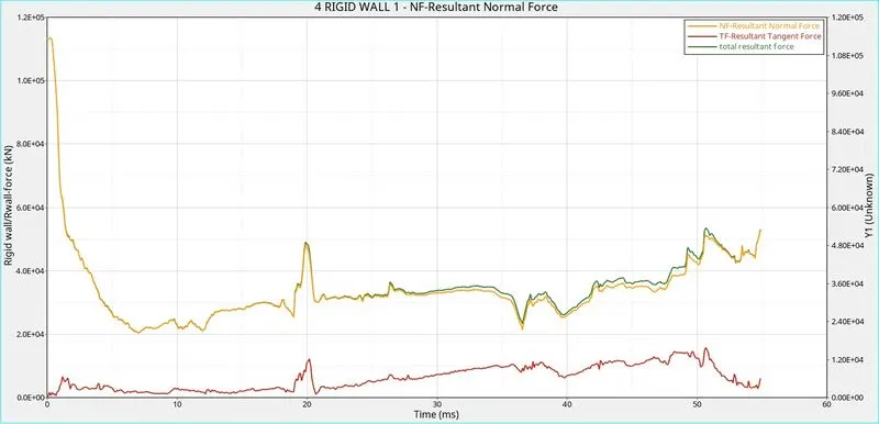
• The above plot shows the total resultant force, resultant normal force, and resultant tangent force.
• The total resultant force is the sum of normal force and the wall's tangential force (frictional force).
• The total resultant force vertical axis is presented on the right side of the graph.

Case 2: Recommended 2D element formulation.

• Change the simulation time from 60ms to 55 ms in the "ENG_RUN" card.

Fig 9: Simulation time is set in the Tstop row.

• For obtaining 25 animation steps for the results, the Tfreq value is changed to 0.9166 (total simulation time/number of animation steps required) in the "ENG_ANIM_DT" card.

Fig 10: Required number of animation steps are set.

Parameters		Comment
Ishell =24		QEPH 4 nodes shells are best combination of cost and accuracy.
Ismstr=2		Full geometric nonlinearities (default)with possible small strain formulation activation in RADIOSS Engine.
Ish3n=2		Standard 3 noded shell (C0)with modification for large rotation(default)
N=5		Number of integration points set to 5 for accuracy bending.
Ithick=1		Thickness change is taken into account for accuracy.
Iplas=1		Iterative plasticity for good accuracy.

• The parameters as mentioned above are set in the property of Hat-section and close-out panel.

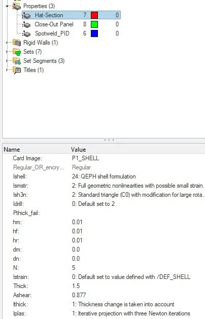
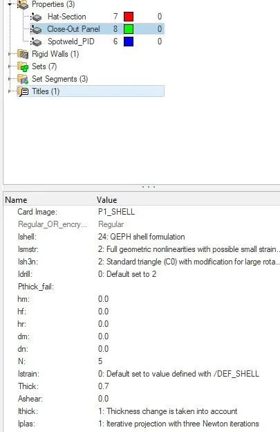
Fig 11: The recommended element values are set in the properties.

• Now we can proceed to run our simulation. Navigate to the analysis tab and choose the radioss option.
• Input file option will be available to save the starter and engine file in the desired location.
• In the options bar, "-nt 6" is entered, which denotes parallel processing for the simulation.
• A separate window pops up and shows the calculation going on, and it might take up to few seconds to minutes based on the complexity of the solution.

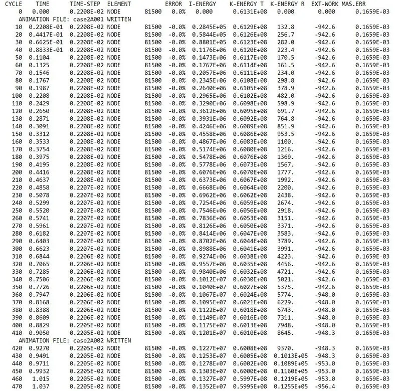
Fig 12: 0001.out files contains the solution information.

• We can check for the energy and mass error from the engine output file whether it lies within the permissible limit or not.
• The energy error starts from -0 to -10%, and the mass error is 0.1659E-03. Both are in the acceptable range, and we can proceed with the post-processing of our results.

Results:

• For post-processing the results Hyperview and hypergraph are used.
• When hyperview is open, we need to load the model and results file of our simulation.

Fig 13: Loaded result file.

• To visualize the contours, we navigate to the contour option, in which we have multiple options to see the results.

Fig 14: Contour options.

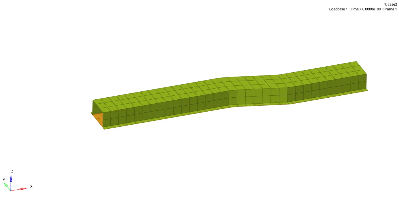
• The above animation represents the crash of rail to the rigid wall (the rigid wall is hidden for better view).

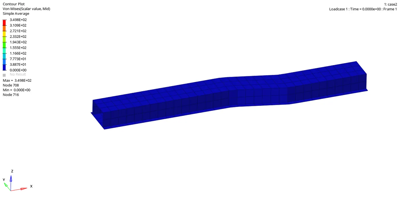
• The above animation represents the von mises stresses generated in the rail.

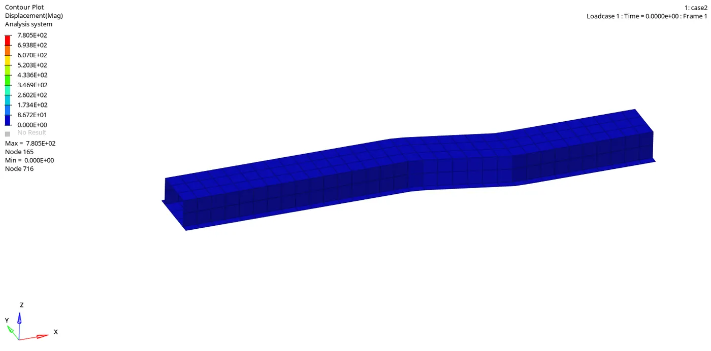
• The above animation represents the displacement produced in the rail.

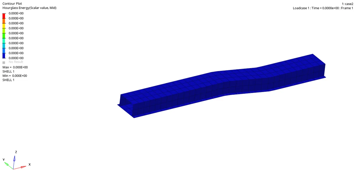
• The above animation shows the hourglass energy.

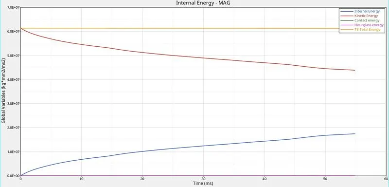
• The above plot shows the Total energy, Kinetic energy, Internal energy, hourglass energy, and contact energy.
• The total energy is the summation of an internal, kinetic, hourglass, and contact energy.
• Kinetic energy initially is higher because the system moves with a certain velocity and is hitting the rigid wall, as the model crashes the wall and finally comes to rest, so the kinetic energy decreases as the simulation goes on.
• Internal energy is the sum of kinetic and potential energy in a system.
• Contact energy is formed because the rail comes in contact with the rigid wall, and the connection between them is the same throughout the simulation.

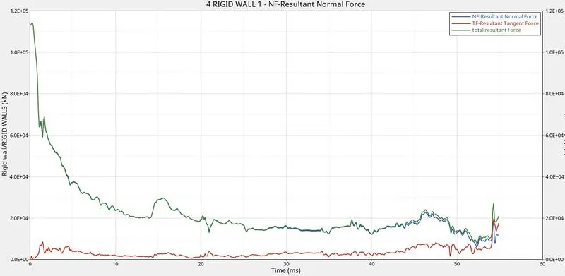
• The above plot shows the total resultant force, resultant normal force, and resultant tangent force.
• The total resultant force is the sum of normal force and the wall's tangential force (frictional force).
• The total resultant force vertical axis is presented on the right side of the graph.

Results discussion with a comparison of Case1 and Case2:

• Observing the crash onto the rigid wall, the final shapes acquired by case 1 and case 2 are entirely different.
• The maximum Von Mises stresses generated in both the case are the same,i.e., 3.498E+02.
• The maximum displacement generated in both cases is different by a considerable margin. Case 1 produces a displacement of 8.574E+02, whereas case 2 produces 7.805E+02.

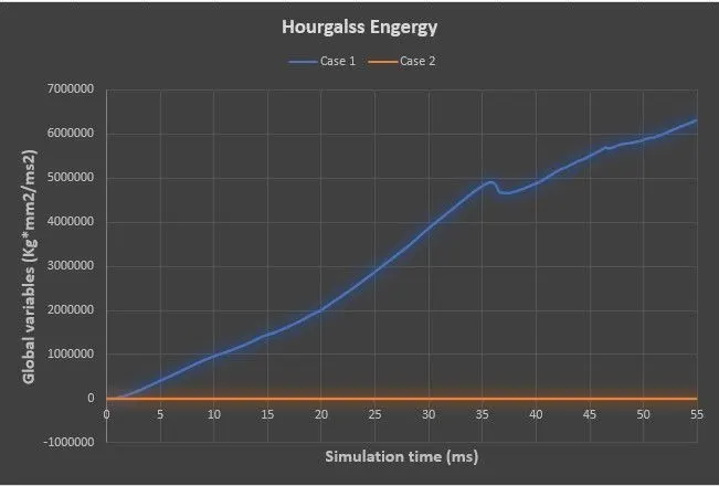
• The above graph clearly shows the hourglass energy produced in each case. In case 2, because of QEPH elements, the hourglass is perfectly controlled with additional stiffness in the elements. While in case 1 with the default element settings, a tremendous amount of hourglass energy was generated in a few of the elements, which resulted in the inaccuracy of the result.
• Also, the total energy throughout the simulation is constant in case 2. In case 1, we can observe a decrease in the total energy, which states there is some extra energy loss in the system.
• The contact energy is different in case 2 when compared with case 1, and that is evident by the shape the rail acquires in both the crash scenarios.

Hourglass energy:

A phenomenon occurs when an element gets deformed in a model, but the strain energy is not calculated. We know stress is calculated from the strain and applied as force onto the next element. When there is no calculation in the strain energy due to the hourglass, the stress will be zero for that particular element. Therefore the following element has zero force applied to it. Because of this inappropriate force flow or distribution in the model, the hourglass must be controlled to get accurate results for the simulation.

Ways to avoid hourglass formation:

• One efficient way is by choosing a proper element property, which has reasonable control over the hourglass energy.
• Adding additional stiffness to the elements balances the hourglass effect.
• Fully integrated elements can be used instead of reduced integration elements, but it is computationally costly.
• Finer mesh controls the hourglass effect efficiently than coarse mesh.

Conclusion: The crash rail was tested under two different element formulation conditions, and their results were compared.