Assignment 3-2D Element Formulation Challenge

Objective

Compare the base simulation and with the improved shell element properties. We have to change the run time to be 55 ms and we have to change the steps of the animation to be between 25 to 60. Check the energy error and mass error. We have to plot the rigid wall forces, internal energy, hourglass energy, contact energy, and total energy.

Procedure

Case-1

Simulation with the default values of the beam file.

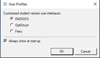
1. We are going to choose the profile to be Radioss.

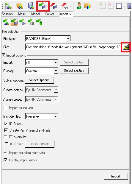
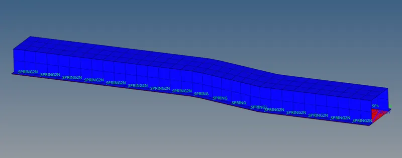
2. Now we are going to import the model.

3. Now we are going to check the unit of the model. For that, we will go to the BEGIN_CARD.

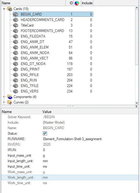
So the unit of the system is in g, mm, ms.

4. Now we are going to change the end time of the simulation. To change that we will go the Cards--> ENG_RUN

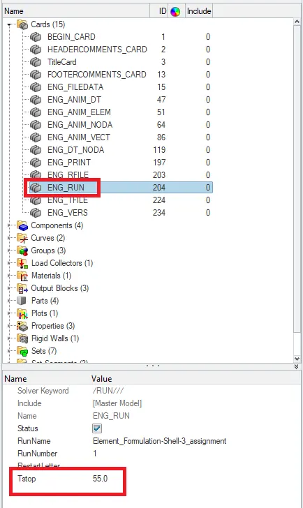
Run time is the time in which we define that for how long we want to run the simulation.

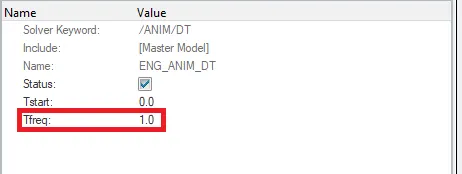
5. Now we have to change the no. of animation steps. We need to take the animation steps to be between 25 to 60. I have taken the animation steps to be 55. To do that we have to change the frequency of the animation. Because the frequency is the ratio of the run time to the no. of the animation file.

`T_("freq")= "Run time"/"No. of animation file"`

So `T_("freq") = 55/55 = 1.0`

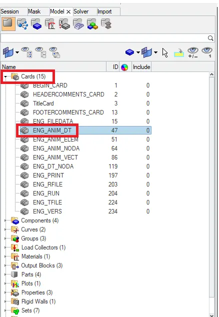
To change the frequency we will go to the Cards--> ENG_ANIM_DT

6. After changing the values we will run the simulation. To run the simulation we will go to the Analysis-->Radioss

7. To check the simulation we have done is correct or not we are going to check the energy error and mass error. If it is in the accepted range then we can say that our simulation is correct.

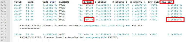
The energy error is less than -15% and the mass error is 0.166e-03. That is very less so we can see that the simulation we have done is right.

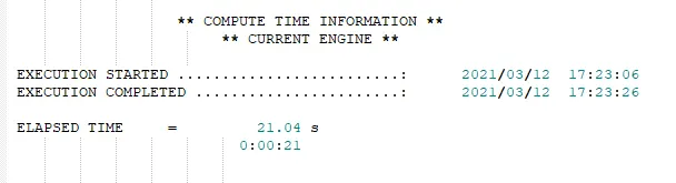
The total running time of the simulation was 21 seconds.

8. Now we are going to analyze the simulation and we are going to plot the required graph.

Output

Simulation Gif

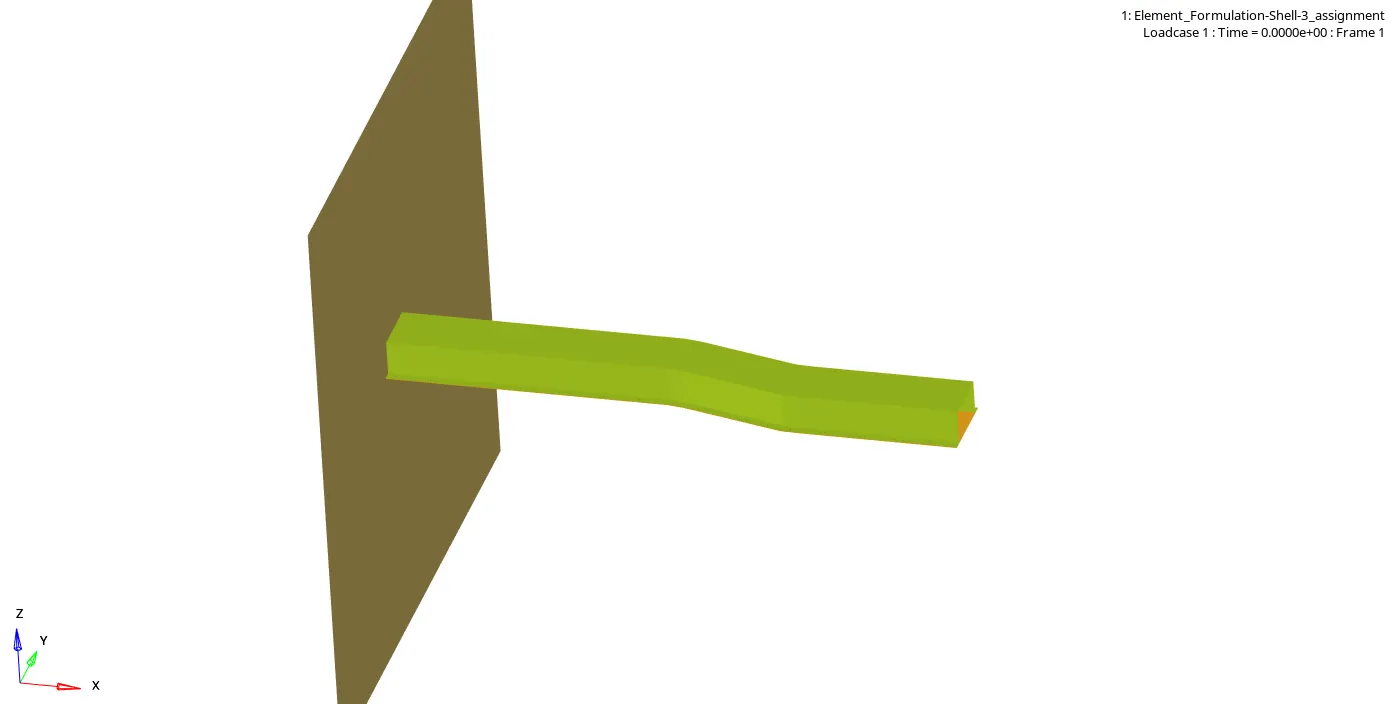
So in the simulation, we can see that the elements are deforming. First, the elements which are in the middle of the beam deformed. After that the elements which are present near the rigid wall deformed.

Displacement Gif

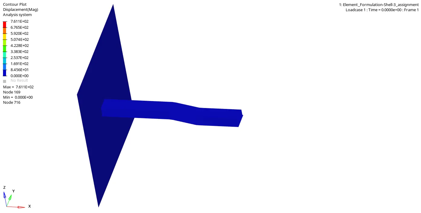
In the simulation, we can see that the elements which are at the rear end of the beam get displaced very much because the direction of the velocity of the beam is in the negative x-direction. So the elements which are near the rigid wall do not get any displacement.

Energy Plot

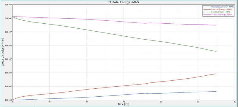
In the above graph, we can see that when the beam gets collides with the rigid wall the velocity of the beam gets decreases because of that the kinetic energy of the beam also get decreases. When the kinetic energy decreases internal energy increases.

We can see that total energy is decreasing with respect to time. So it means that there is some energy that is getting dissipated during the simulation. The decrease in the total energy of the model causing an increase in the hourglass energy.

Hourglass energy 

When the element of the model deformed beyond the deformation limit, in that case, to stabilize the simulation solver add some physical energy that energy is Hourglass energy. 

Contact Energy

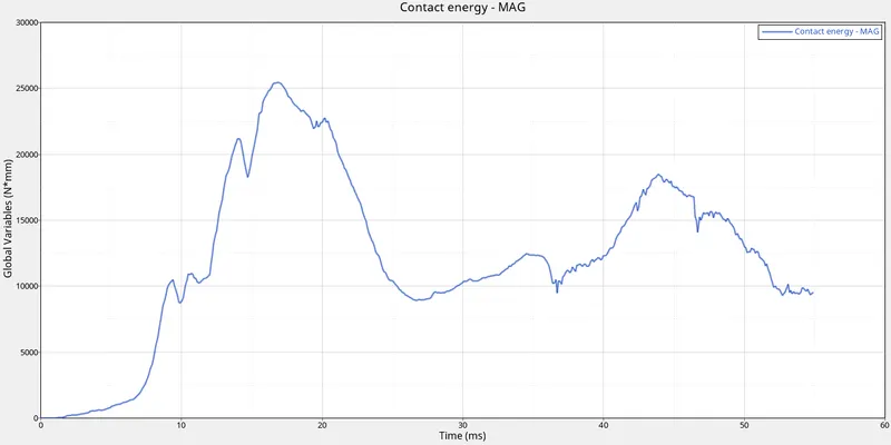
Contact Energy is the energy due to contact between two elements. So when the deformation occurs elements start to get in contact with each other so due to contact between elements we get the contact energy.

In the starting, the contact energy was zero. So when elements start to deformed we get the contact energy. We get the contact energy to be maximum at the 18 ms because at that time the contact between elements was very high after that it reduced. And when the rear elements and front elements get in contact it again increases.

Rigid Wall Forces

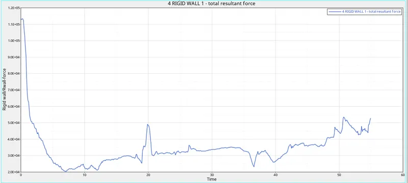
Rigid wall forces are the forces that are acting on the rigid wall by the other object.

In this case, the beam has some velocity and it is going to collides with the rigid wall. In the starting, there is no impact in the simulation but in the graph, we can see that it is showing maximum wall force. It is because at that time there is no record of any force on the rigid body.

So when the tube hits the wall we get the maximum rigid wall force, the solver takes that value for the missing time.

Case-2

Change the shell element properties to recommended properties and run the simulation

1. We are going to choose the profile to be Radioss.

2. Now we are going to import the model.

3. Now we are going to check the unit of the model. For that, we will go to the BEGIN_CARD.

So the unit of the system is in g, mm, ms.

4. Now we are going to change the end time of the simulation. To change that we will go the Cards--> ENG_RUN

Run time is the time in which we define that for how long we want to run the simulation.

5. Now we have to change the no. of animation steps. We need to take the animation steps to be between 25 to 60. I have taken the animation steps to be 55. To do that we have to change the frequency of the animation. Because the frequency is the ratio of the run time to the no. of the animation file.

`T_("freq")= "Run time"/"No. of animation file"`

So `T_("freq") = 55/55 = 1.0`

To change the frequency we will go to the Cards--> ENG_ANIM_DT

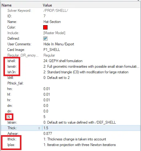
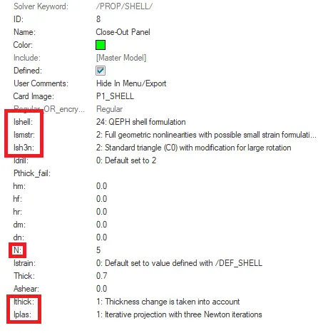
6. Now we are going to change the shell element properties to the recommended properties.

Ishell

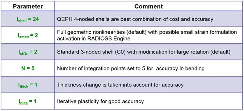
When the thickness of the component is less than 6 mm we convert that component from 3D to 2D. So in that case we take the shell elements. So Ishell is the 2D representation of the 4 noded elements in the RADIOSS.

The recommended value of Ishell is Ishell =24. It is a QEPH type of element. Which is an improved under-integrated element. In this type of shell element, the integration point on the surfaces decreases. WHich decreases our computational time. 

It uses the stiffness method which is a physical hourglass stabilization. So when the deformation goes beyond the limit. It increases the stiffness of the element. So that the simulation does not get unstable. 

Ismstr

Ismstr is the small strain formulation. It goes activated when the element starts to deform. It stored the strain value of the elements. 

The recommended value of the Ismstr is Ismstr = 2. When the elements get a large deformation/strain. It will switch to the large strain.

Ish3n

Ish3n is the representation of the 3 noded elements in the RADIOSS.

The recommended value of the Ish3n is Ish3n = 2. It is a standard triangle with modification for large rotation. It has only 1 integration point on the surface. There is hourglass deformation.

N

N is the no. of integration points we want through the thickness of the element. We can give the no. of integration points to be up to 10.

The recommended value of N is 5. When we take N to be 5 we get the accuracy with less cost.

Ithick

So when the elements start to deform, the thickness of the elements also changes. So we need to choose that if we want to take that change of the thickness into account or not.

The recommended value of the Ish3n is Ithick = 1. Which is that we have to take the change in the thickness to be in the account. Which gives us an accurate result.

 Iplas

When the elements go beyond the elastic region and go to the plastic region it goes activated.

The recommended value of the Ish3n is Iplas = 1. When the elements go to the plastic region. It will calculate the values for the three iterations and give us the average value. It increases the simulation time but we will get the accurate result.

So in order to change the element property. We will go to the property 

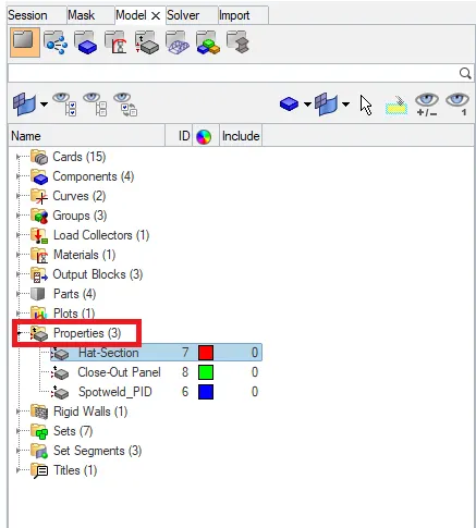
Here we will change the property to the recommended values.

7. After changing the values we will run the simulation. To run the simulation we will go to the Analysis-->Radioss

8. To check the simulation we have done is correct or not we are going to check the energy error and mass error. If it is in the accepted range then we can say that our simulation is correct.

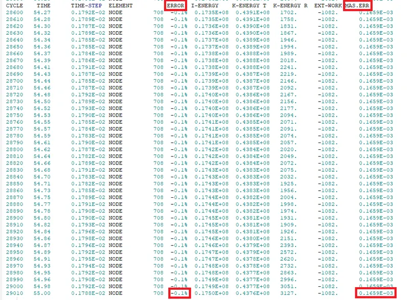
The energy error is less than -15% and the mass error is 0.166e-03. That is very less so we can see that the simulation we have done is right.

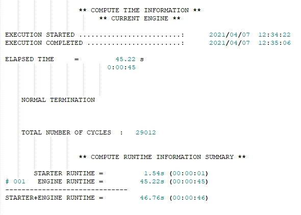
The total running time of the simulation was 46 seconds.

9. Now we are going to analyze the simulation and we are going to plot the required graph.

Output

Simulation Gif

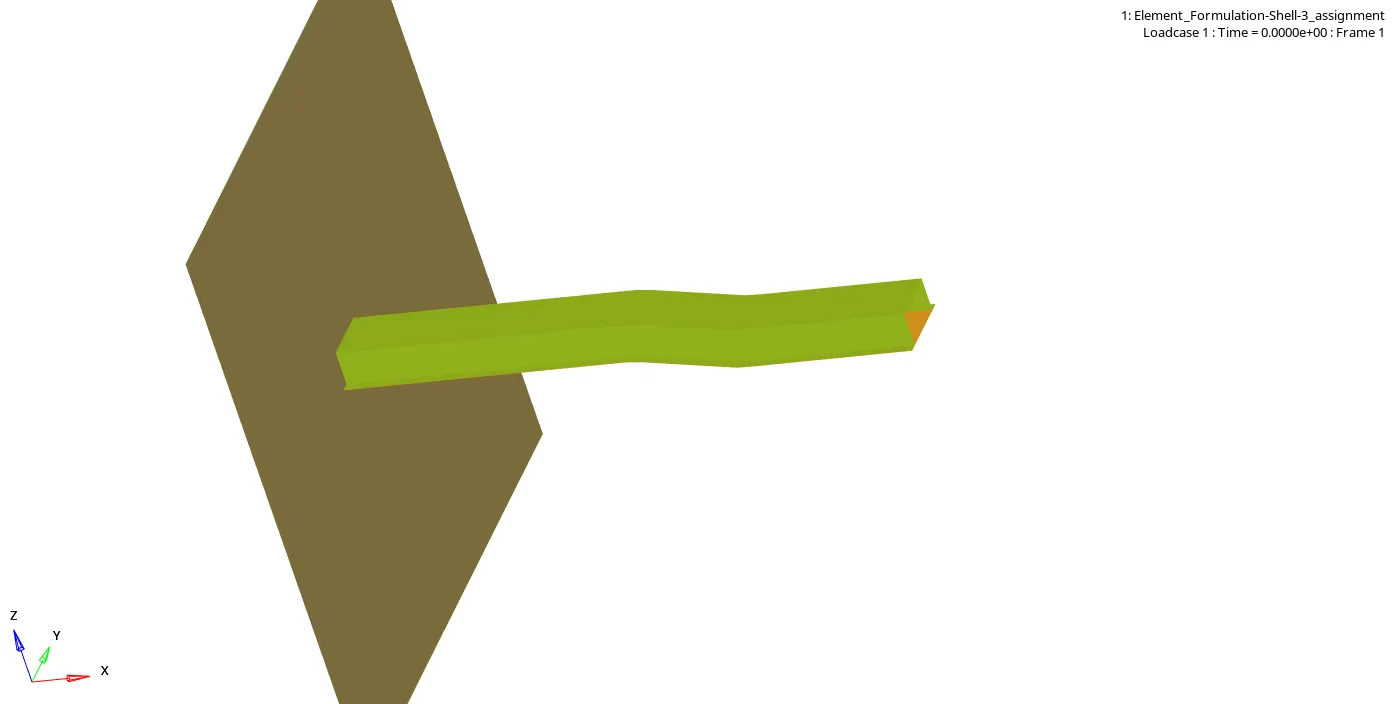
So in the simulation, we can see that the elements are deforming. First, the elements which are in the middle of the beam deformed. After that the elements which are present near the rigid wall deformed.

Displacement Gif

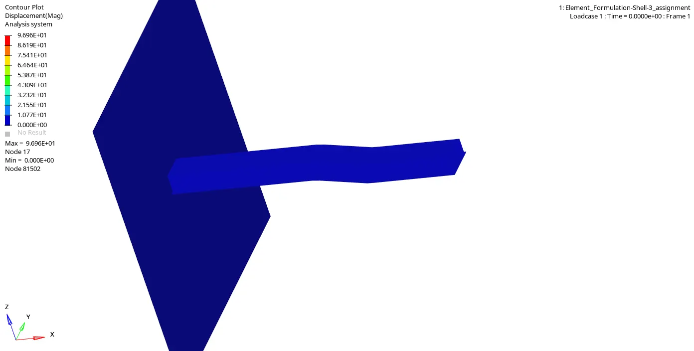
In the simulation, we can see that the elements which are at the rear end of the beam get displaced very much because the direction of the velocity of the beam is in the negative x-direction. So the elements which are near the rigid wall do not get any displacement.

Energy Plot

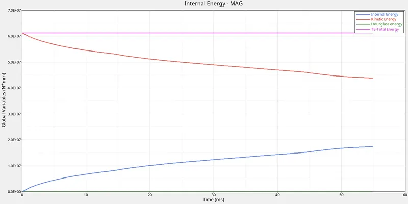
In the above graph, we can see that when the beam gets collides with the rigid wall the velocity of the beam gets decreases because of that the kinetic energy of the beam also get decreases. When the kinetic energy decreases internal energy increases.

We have taken the QEPH element. So the hourglass energy we got is zero.

Contact Energy

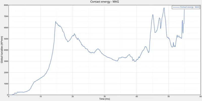
Contact Energy is the energy due to contact between two elements. So when the deformation occurs elements start to get in contact with each other so due to contact between elements we get the contact energy.

In the starting, the contact energy was zero. So when elements start to deformed we get the contact energy. We get the contact energy to be maximum at the 12 ms because at that time the contact between elements was very high after that it reduced. And when the rear elements and front elements get in contact it again increases.

Rigid Wall Forces

 

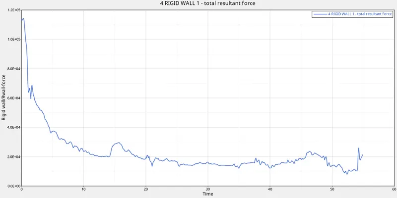
Rigid wall forces are the forces that are acting on the rigid wall by the other object. In this case, the beam has some velocity and it is going to collides with the rigid wall. In the starting, there is no impact in the simulation but in the graph, we can see that it is showing maximum wall force. It is because at that time there is no record of any force on the rigid body.

So when the tube hits the wall we get the maximum rigid wall force, the solver takes that value for the missing time.

Comparision

When we check the simulation of both cases we can see that the deformation of the elements does not make any sense in the first case. The deformation of the element is not proper in the first case. The deformation of the elements in the second case looks more real as compared to the first case. 

In the second case, we have taken the QEPH elements so the hourglass energy we are getting is zero in this case. So total energy was almost constant in this case. It decreases because of the increase in contact energy.

But we get the hourglass energy in the first case. Because of that our total energy get decreases in the first case.

The energy error was way higher in the first case as compared to the second case.

The contact energy is high in the first case as compared to the second case. Contact energy is not good in any case. It is the dissipation of the energy because of the contact between elements.

In the first case, we get the wall forces very high as compared to the second case. 

When we use the recommended properties for the shell elements, the simulation time get increases very much. It almost gets twice in the second case.

Learning Outcome:-

Learn about the shell element properties.

Learn about contact energy, hourglass energy.

Learn about rigid wall forces.

Learn how to create the graphs and save Gif files in the HyperWork.