Assignment 3-2D Element Formulation Challenge
Objective:
1.Using the crash beam file from the previous assignment, change the run time to 55 ms.
2. Change the number of animation steps during simulation to a minimum of 25 and maximum of 60.
3. Run the base simulation without any modification to element properties.
4. At the end of the simulation, do the energy error and mass error checks and determine whether results would be acceptable.
5. If acceptable, Plot rigid wall forces, internal energy, hourglass energy, contact energy, total energy of the simulations.
6. Change all the shell elements properties to recommended properties, save this as separate, rad files and run the simulation.
7. Follow steps 5 and 6.
8. Create a brief report comparing all the results from steps 5 and 6 for both simulations.
9. Comment whether there is any change in the results and why there is any change in the result.
Procedure:
Case 1
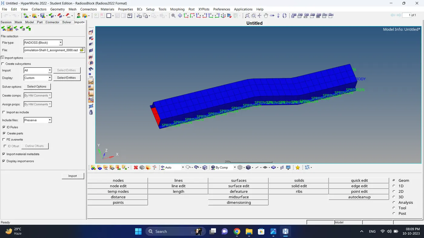
1. Open the Element_Formulation-Shell-3_assignment_0000.rad file in hypermesh.
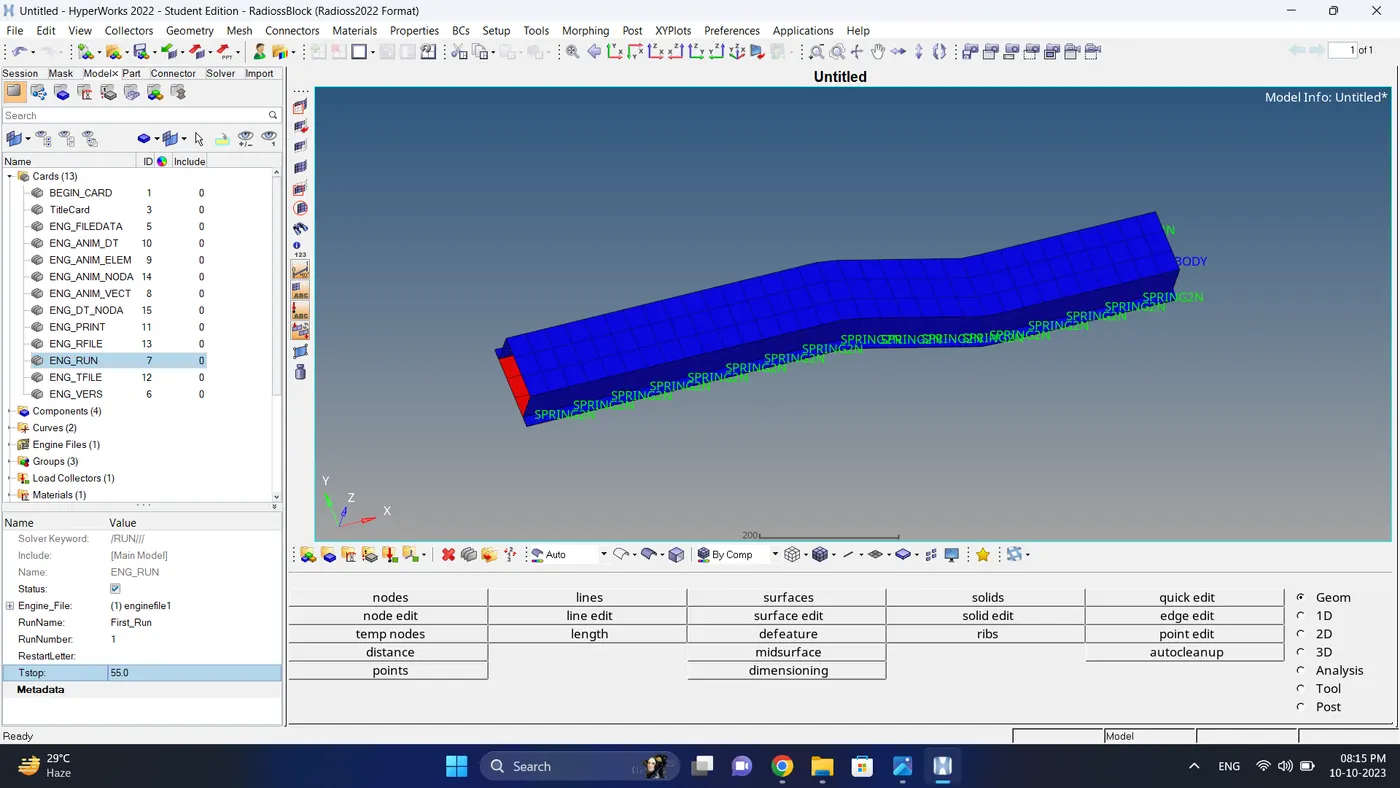
2. To change the run time go to the hypermesh model browser - Expand Cards - Click ENG_RUN - Change Tstop valve to the run time.
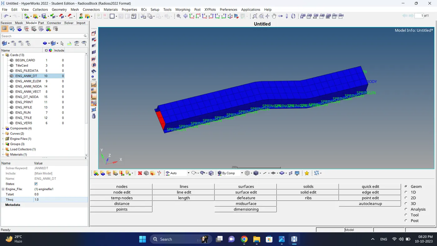
3. Assume the Animation step is 55. i.e T freq = 55/55 = 1
Go to the hypermesh model browser - Expand Cards - Click ENG_ANIM_DT - Change T freq valve to 1.
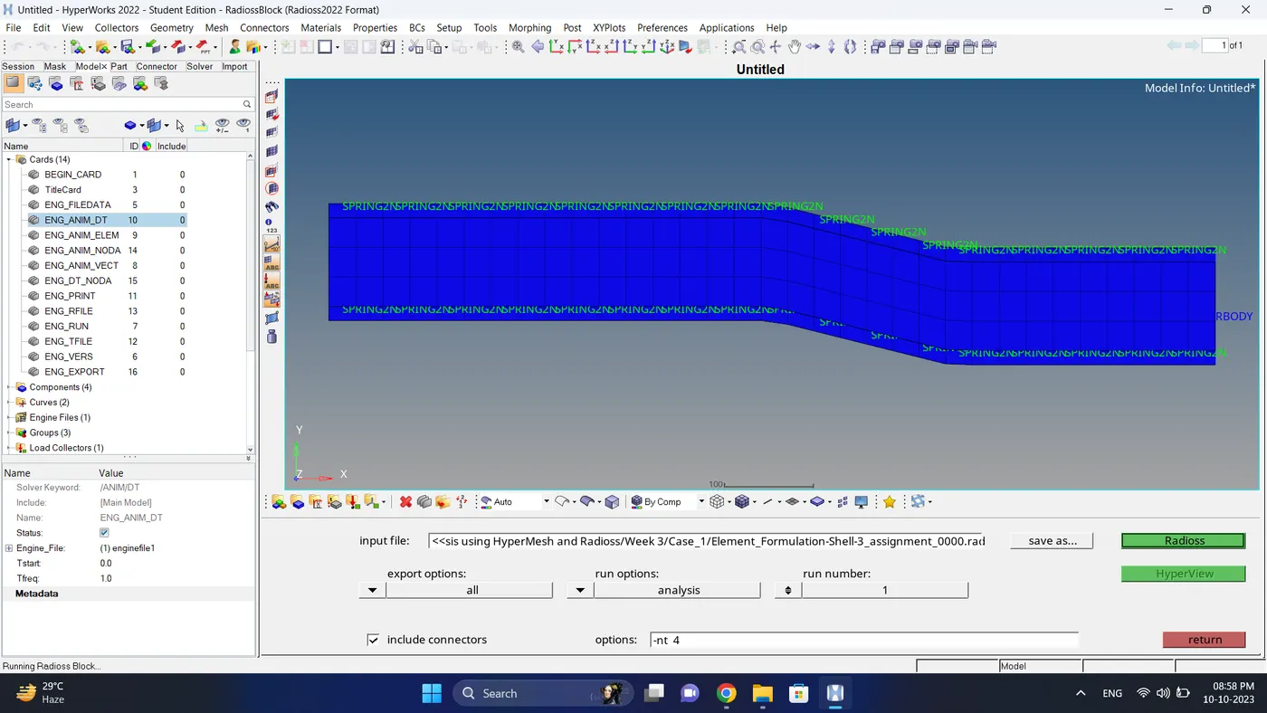
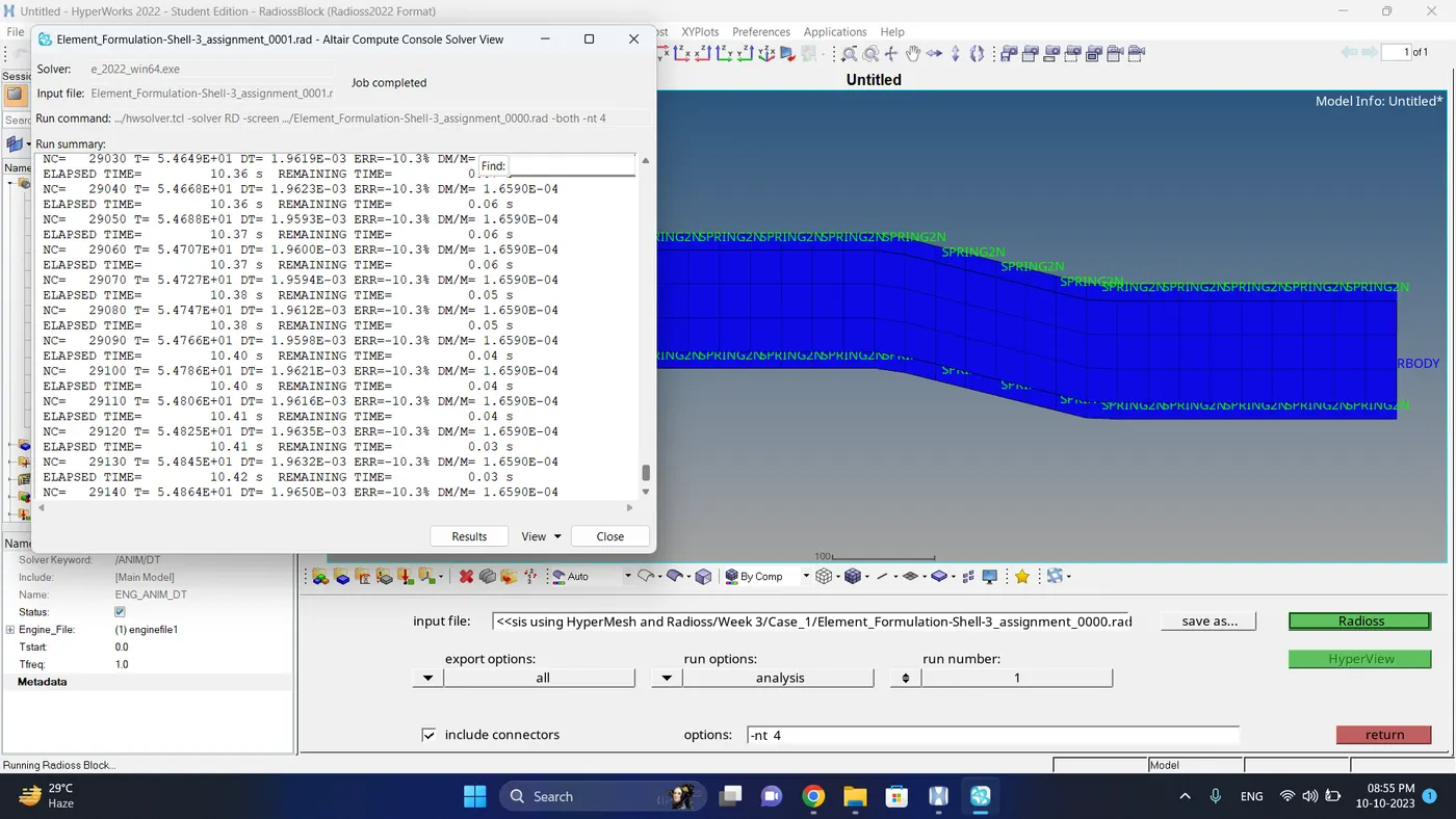
4. Run the simulation.
Go to Analysis - Radioss - click on save as, Rename the file name and at the end type .rad - Ensure that export option is set to all and Include connectors is tick - Click Radioss to run the simulation.
Note: If the stimulation is not running it taking time then copy the given input 0000.rad and 0001.rad file to folder, click on the 0000.rad file click save and overwrite it.
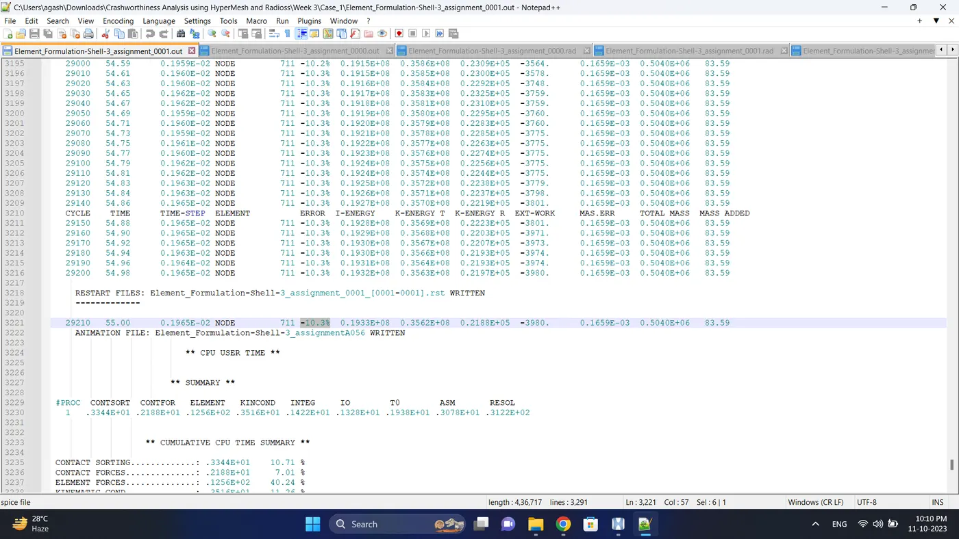
5. Open 0001.out file in notepad ++ and check the maximum total energy error and mass error.
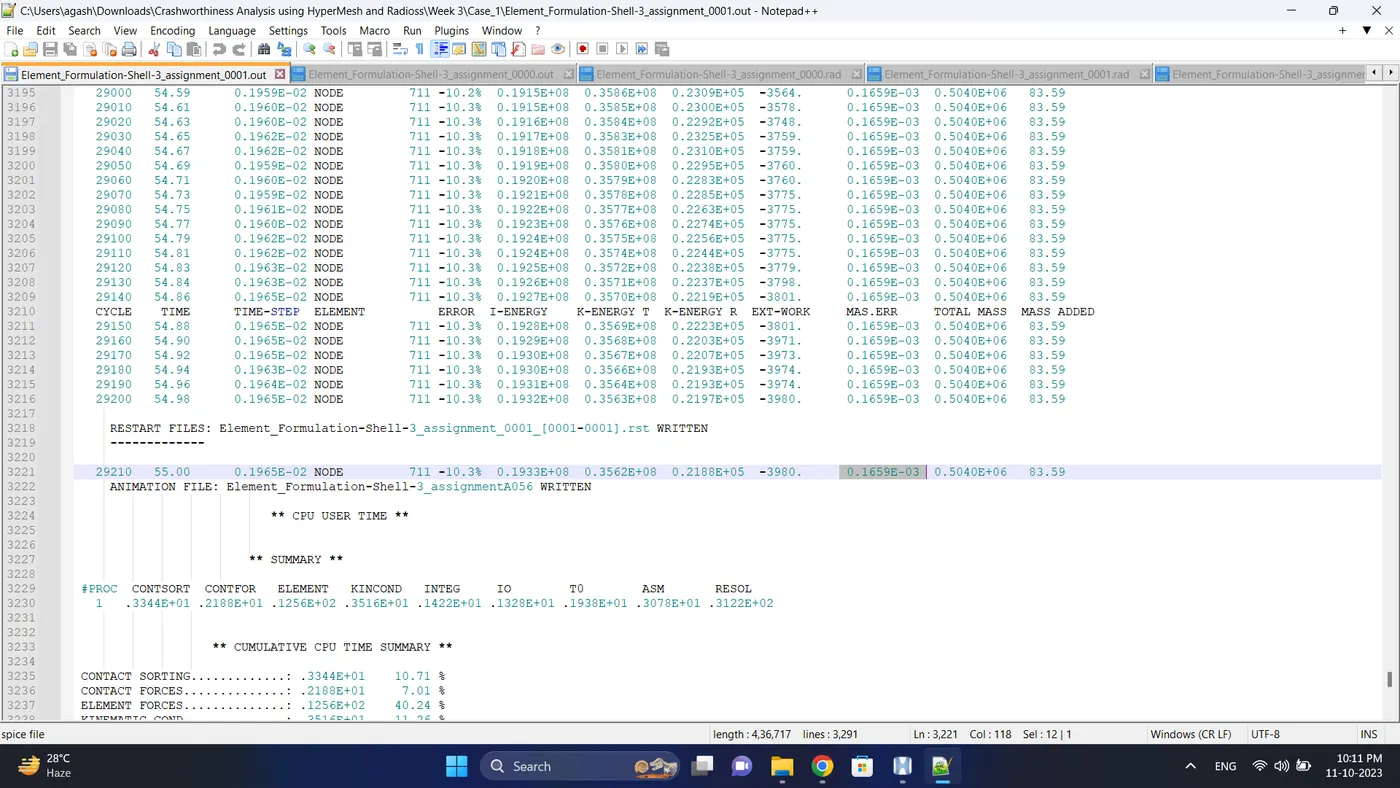
The torelance for the energy error is -15 to +5 % and mass error is upto 2 %
Energy error is -10.3 %
Mass error is 0.1659E-03 (0.0001659) %
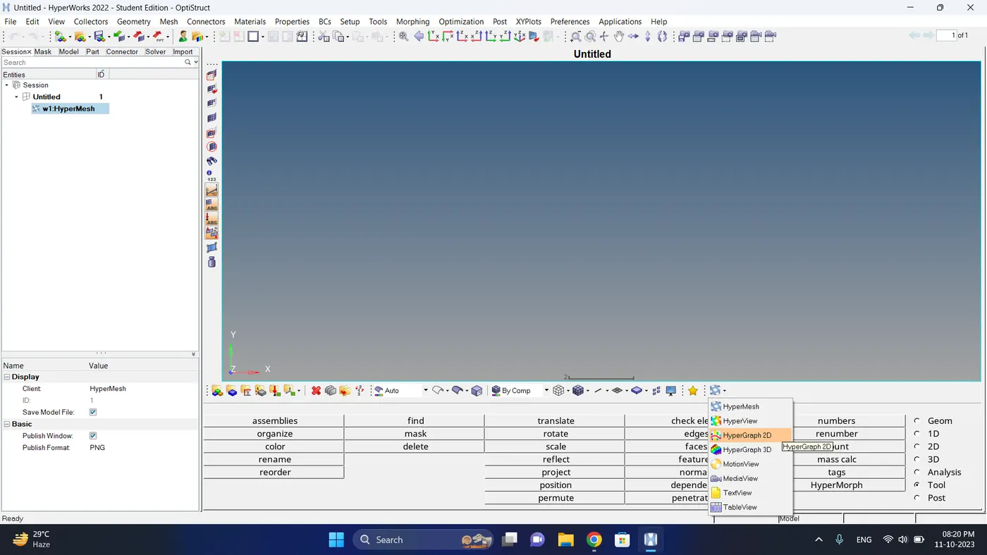
6. Open the Hyperwork in Hypergraph 2D view.
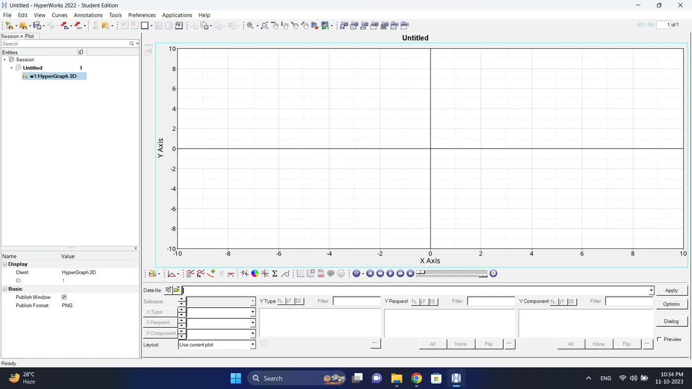
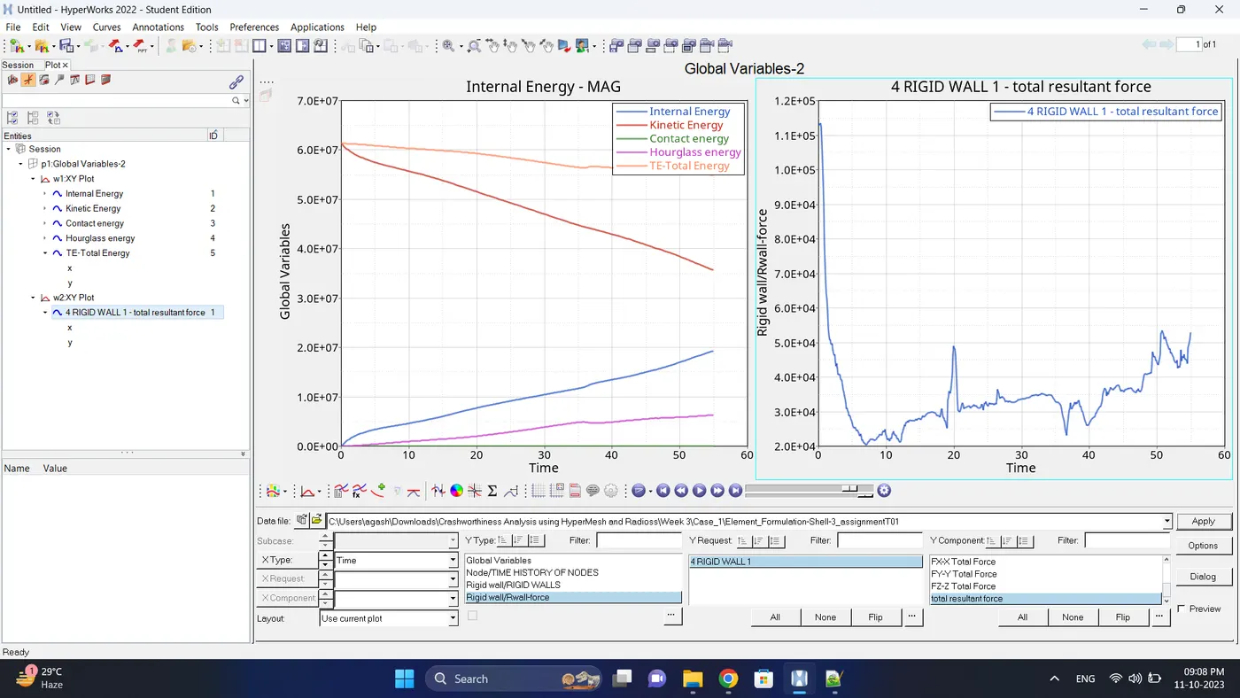
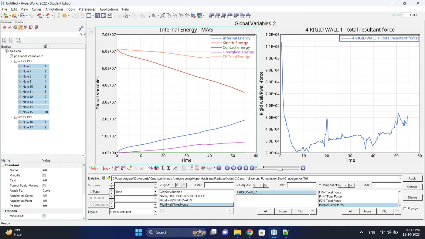
7. Open the T01 file from case_1 and select the Global Variable - Internal energy, Kinetic energy, Contact Energy, Hourglass Energy and Total Energy - Click apply to plot the graph.
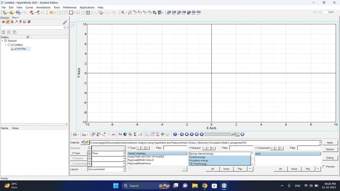
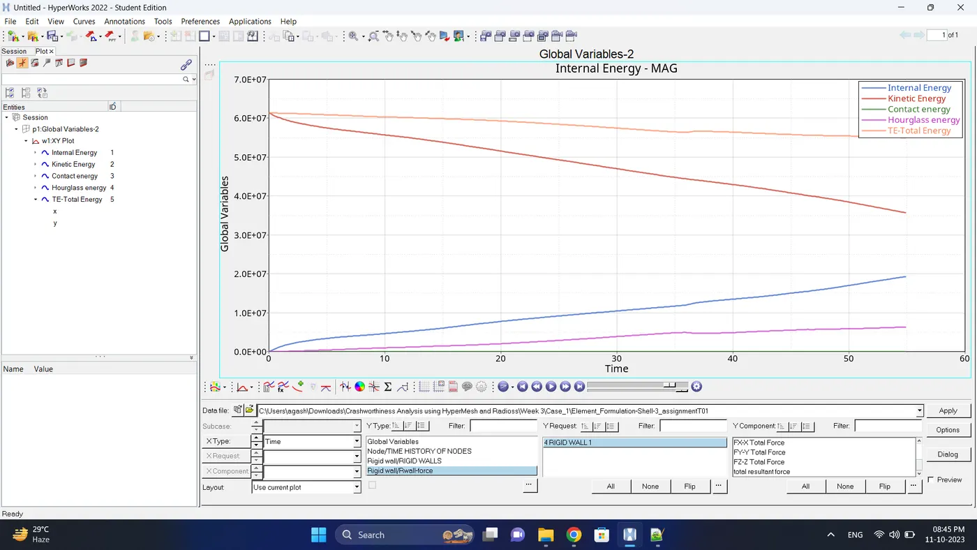
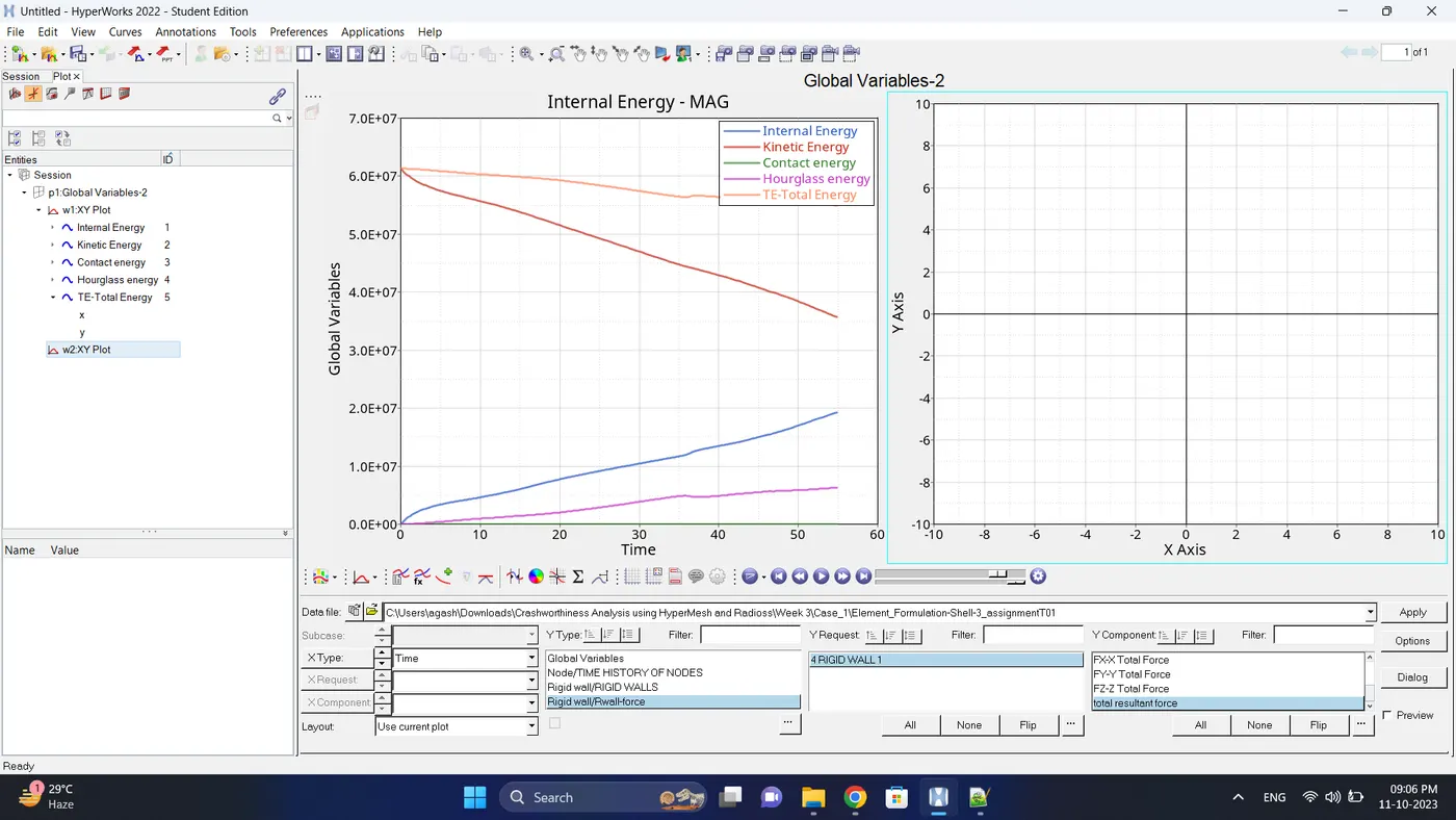
8. Change the windows page layout to 2 and in second window plot the rigid wall forces graph.
To plot graph select, Rigid wall/Rwall-forces - 4 RIGID WALL 1 - total resultant force.
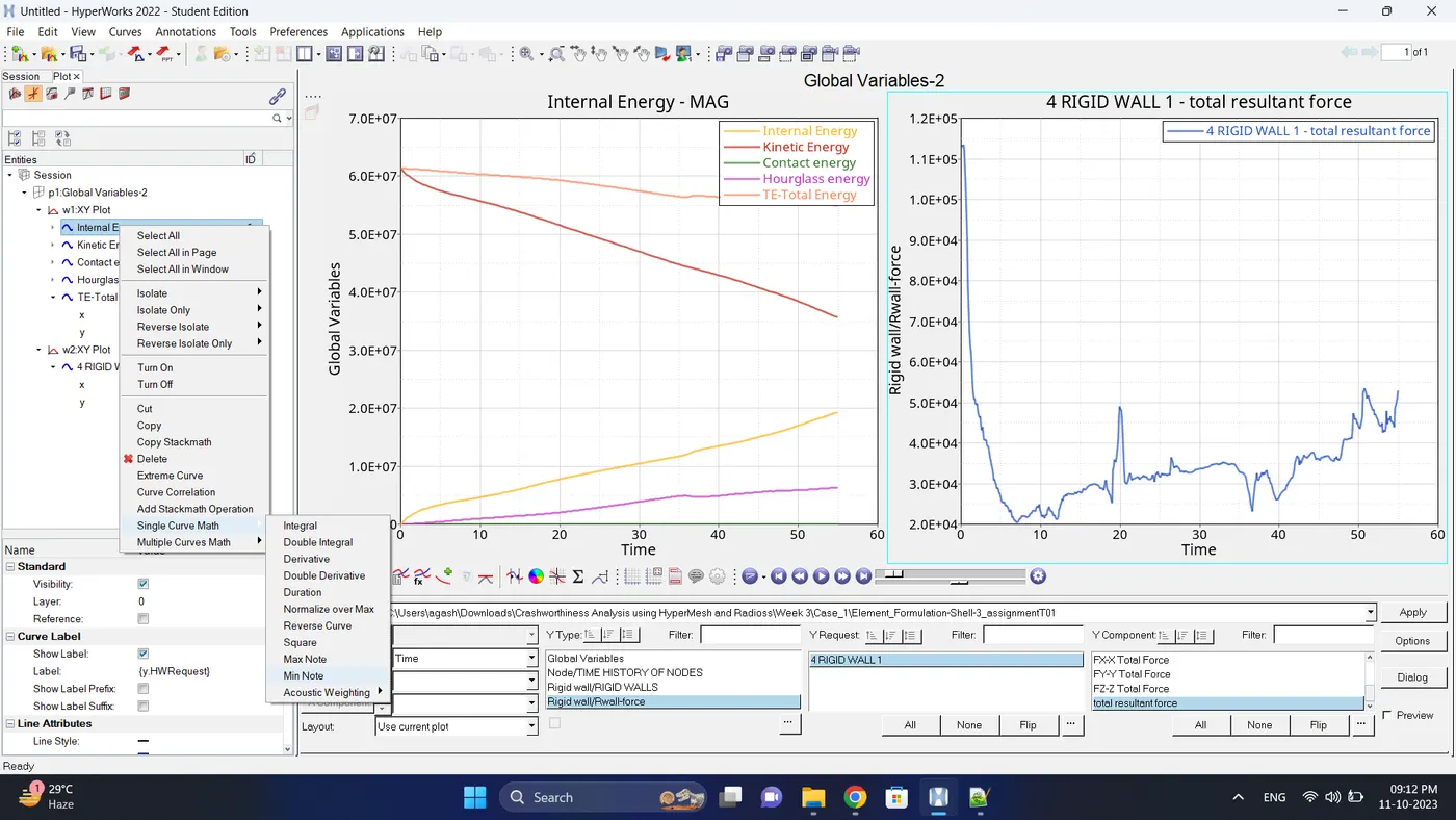
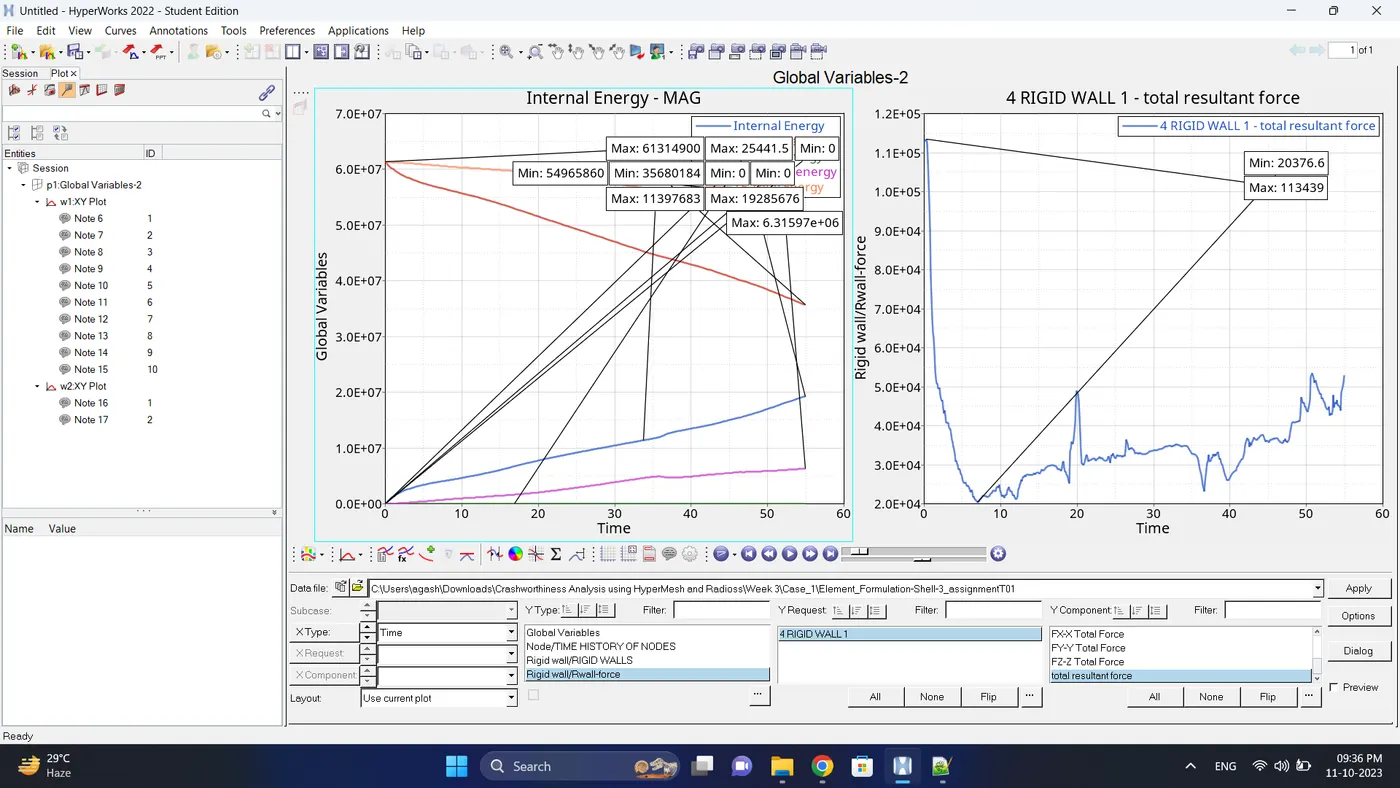
9. Note down the minimum and maximum value of various Energy and forces graph by right click on any energy - Single curve math - Min Note. similarly do for maximum
Note: after getting graph reading turn off that graph and do next reading.
| Sr no. | Name | Minimum | Maximum |
| 1 | Internal Energy | 0 | 19285676 |
| 2 | Kinetic Energy | 35680184 | 61314900 |
| 3 | Contact Energy | 0 | 25441.5 |
| 4 | Hourglass Energy | 0 | 6.31597e+06 |
| 5 | Total Energy | 54965860 | 61314900 |
| 6 | Rigid Wall Force (Total Resultant Force) | 20376.6 | 113439 |
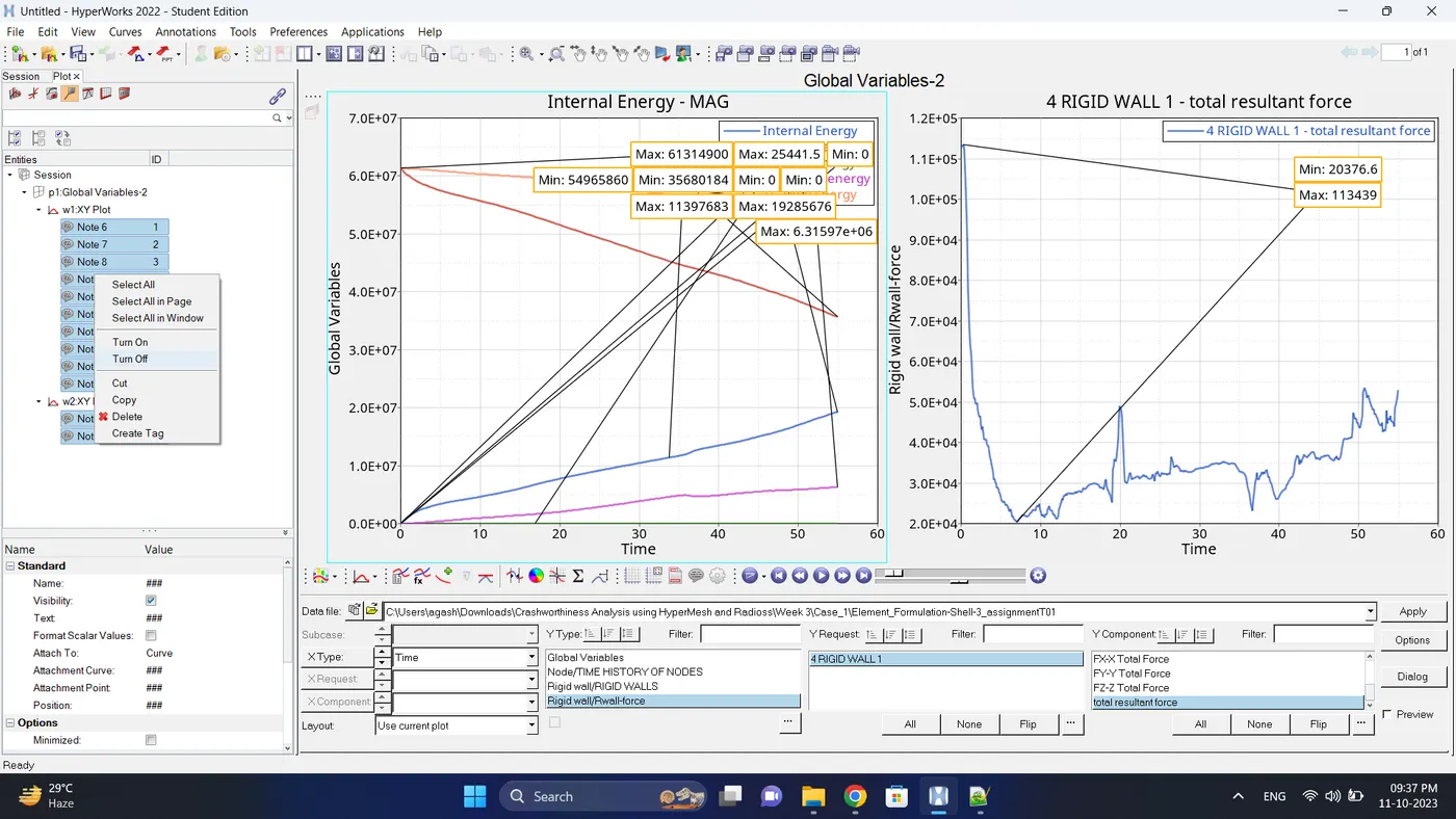
10. After getting all the reading turn off the notes that are plot on graph
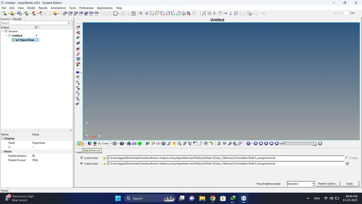
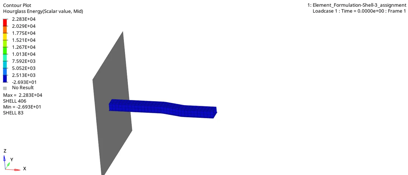
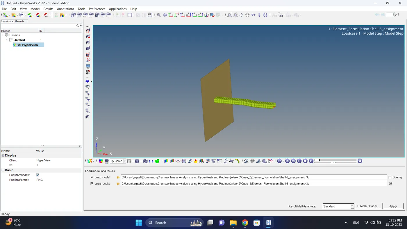
11. Change the view to the Hyperview and load the case_1 .h3d file.
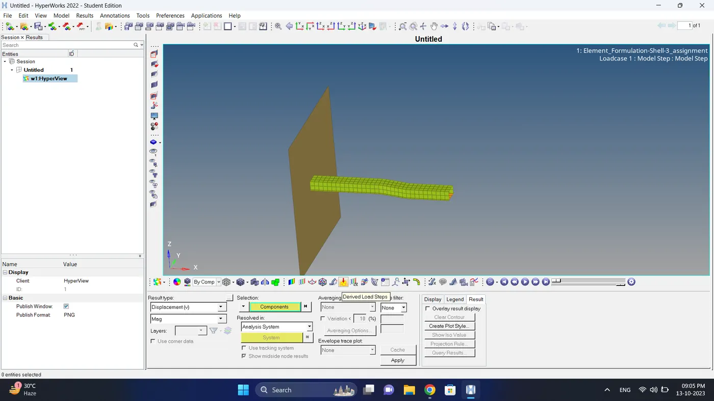
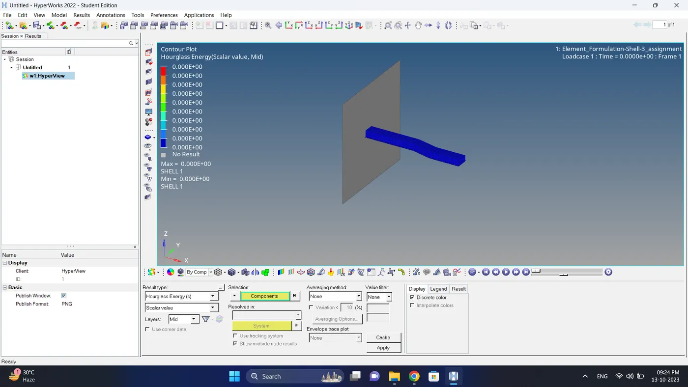
12. Go to Contour - Select Result type to 'Hourglass Energy' - Click Apply.
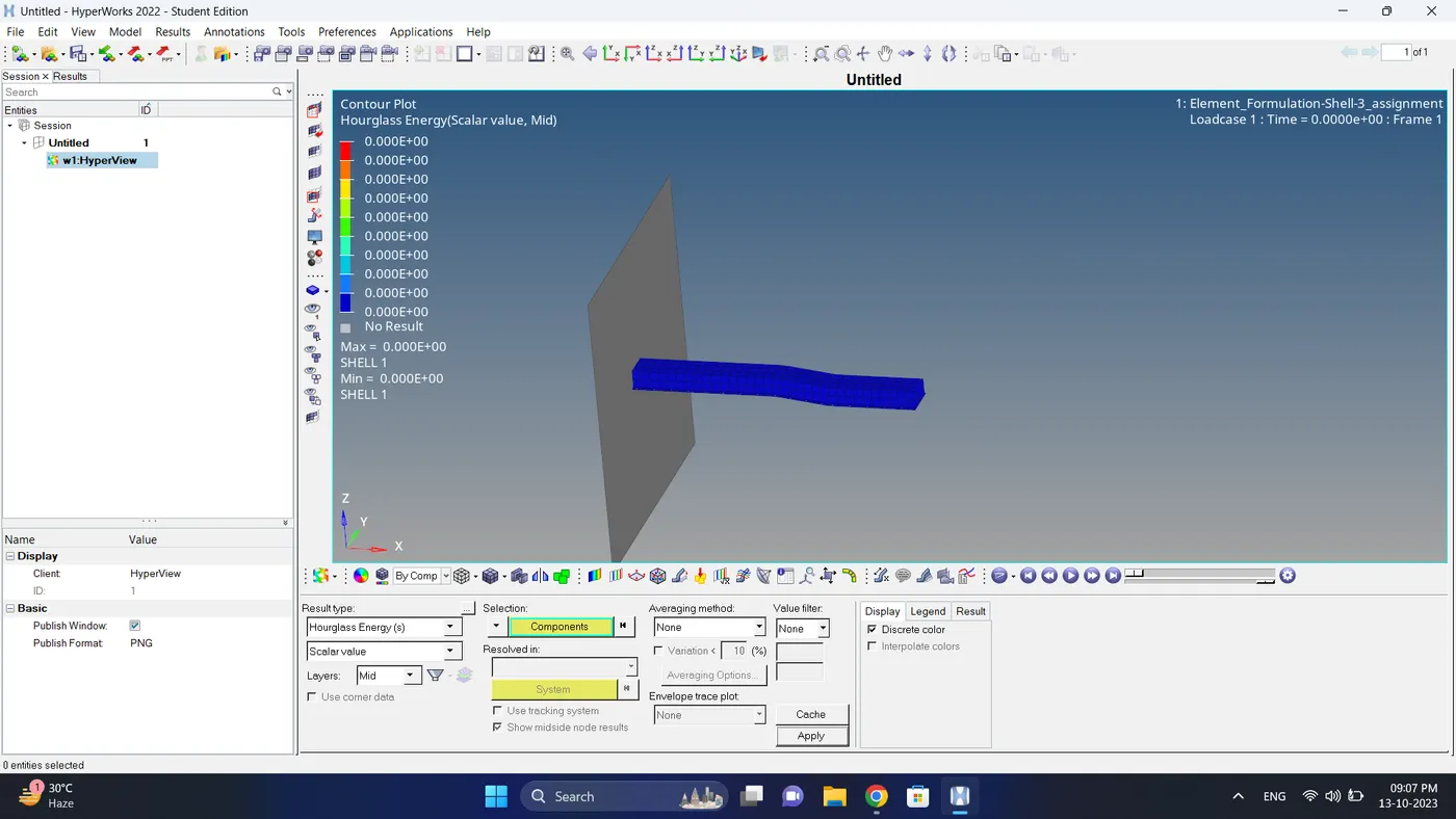
13. Click play to run the animation.
Case 2
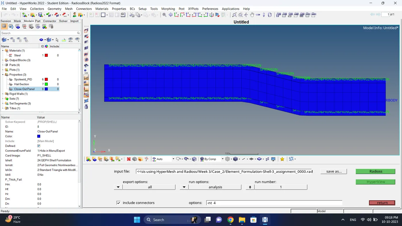
1. After running case 1 simulation in that same file edit shell element material property to the recommended properties.
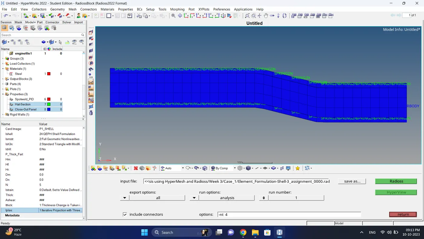
2. After that save the simulation file to another folder and run the simulation.
Note: If the stimulation is not running it taking time then copy the given input 0000.rad and 0001.rad file to folder, click on the 0000.rad file click save and overwrite it.
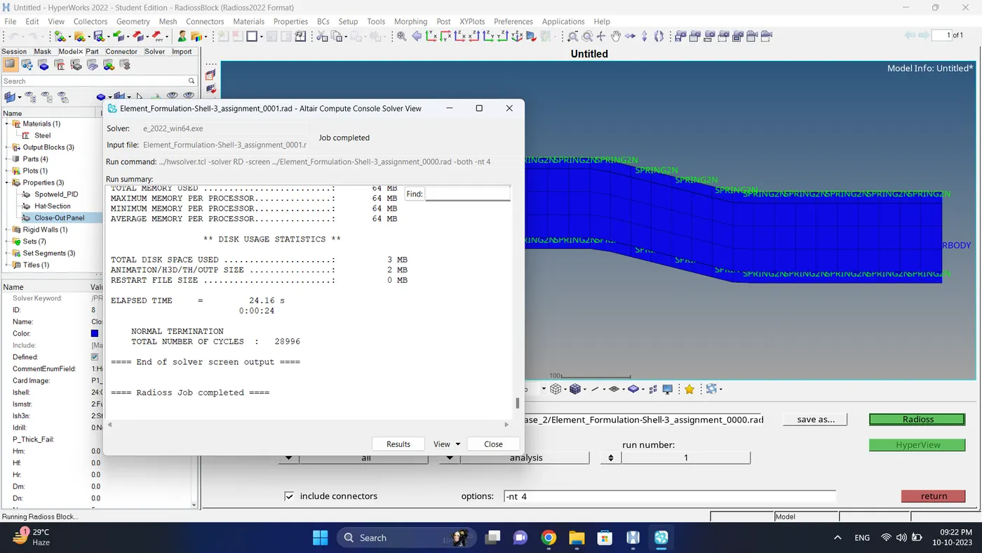
3.Open 0001.out file in notepad ++ and check the maximum total energy error and mass error.
The torelance for the energy error is -15 to +5 % and mass error is upto 2 %
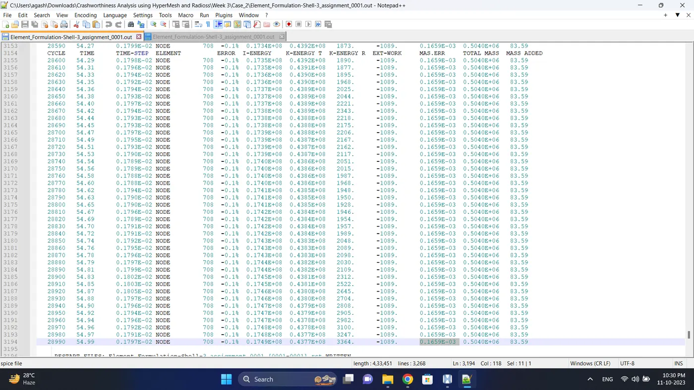
Energy error is -0.1 %
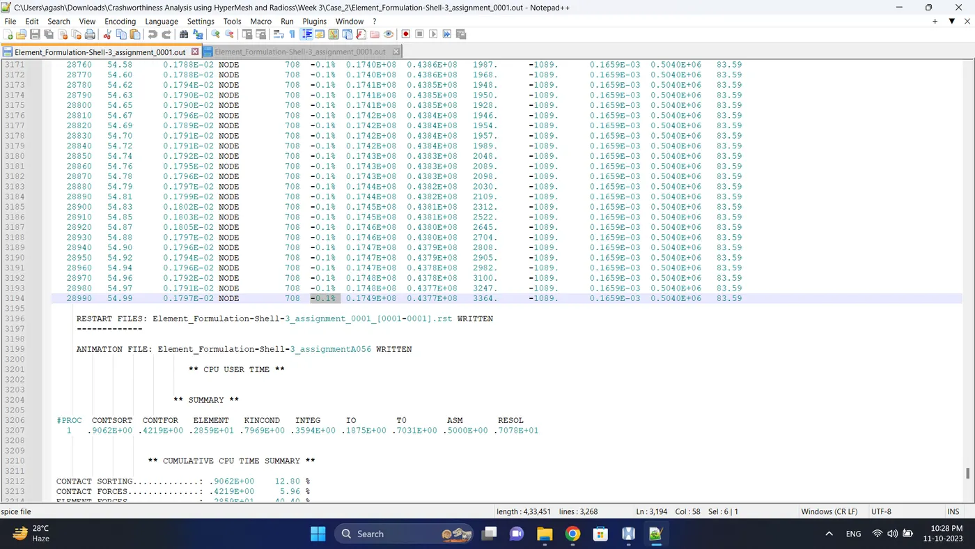
Mass error is 0.1659E-03 (0.0001659) %
4. Open the Hyperwork in Hypergraph 2D view.
5. Open the T01 file from case_2 and select the Global Variable - Internal energy, Kinetic energy, Contact Energy, Hourglass Energy and Total Energy - Click apply to plot the graph.
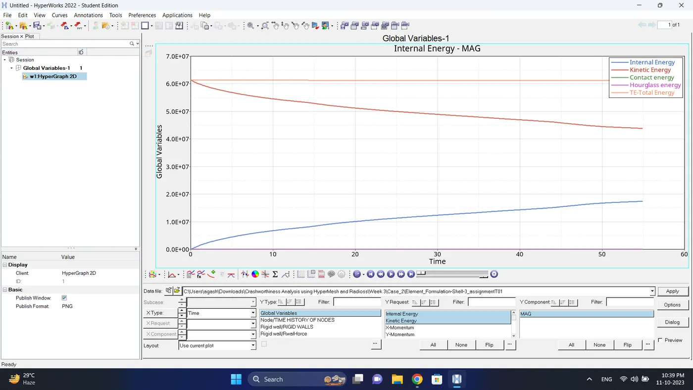
6. Change the windows page layout to 2 and in second window plot the rigid wall forces graph.
To plot graph select, Rigid wall/Rwall-forces - 4 RIGID WALL 1 - total resultant force.
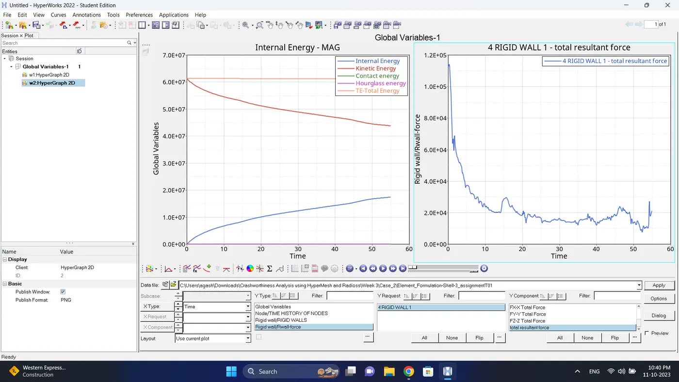
7. Note down the minimum and maximum value of various Energy and forces graph by right click on any energy - Single curve math - Min Note. similarly do for maximum
Note: after getting graph reading turn off that graph and do next reading.
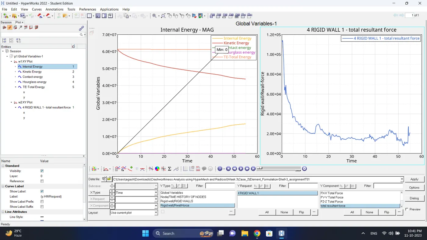
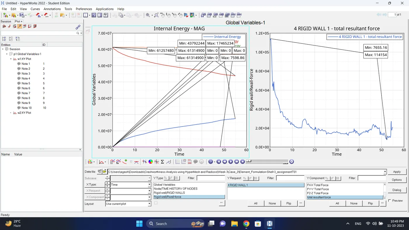
| Sr no. | Name | Minimum | Maximum |
| 1 | Internal Energy | 0 | 17465234 |
| 2 | Kinetic Energy | 43792244 | 61314900 |
| 3 | Contact Energy | 0 | 7598.86 |
| 4 | Hourglass Energy | 0 | 0 |
| 5 | Total Energy | 61257480 | 61314900 |
| 6 | Rigid Wall Force (Total Resultant Force) | 7655.16 | 114154 |
8. After getting all the reading turn off the notes that are plot on graph
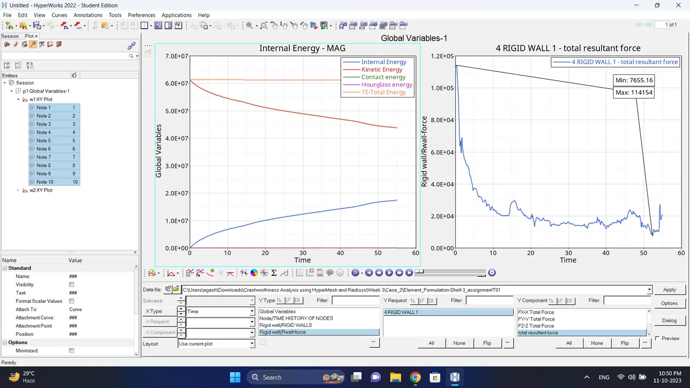
9. Change the view to the Hyperview and load the case_1 .h3d file.
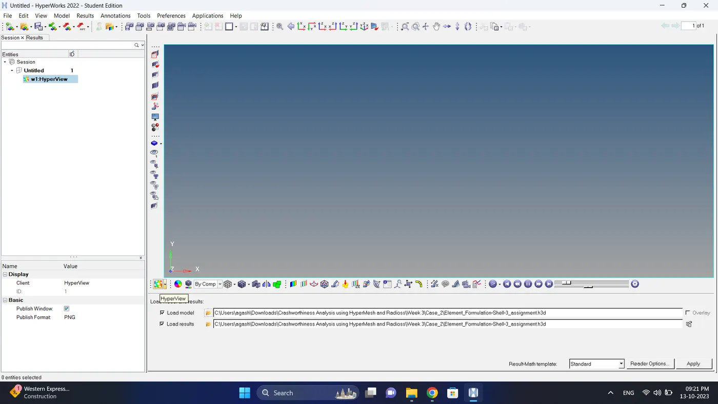
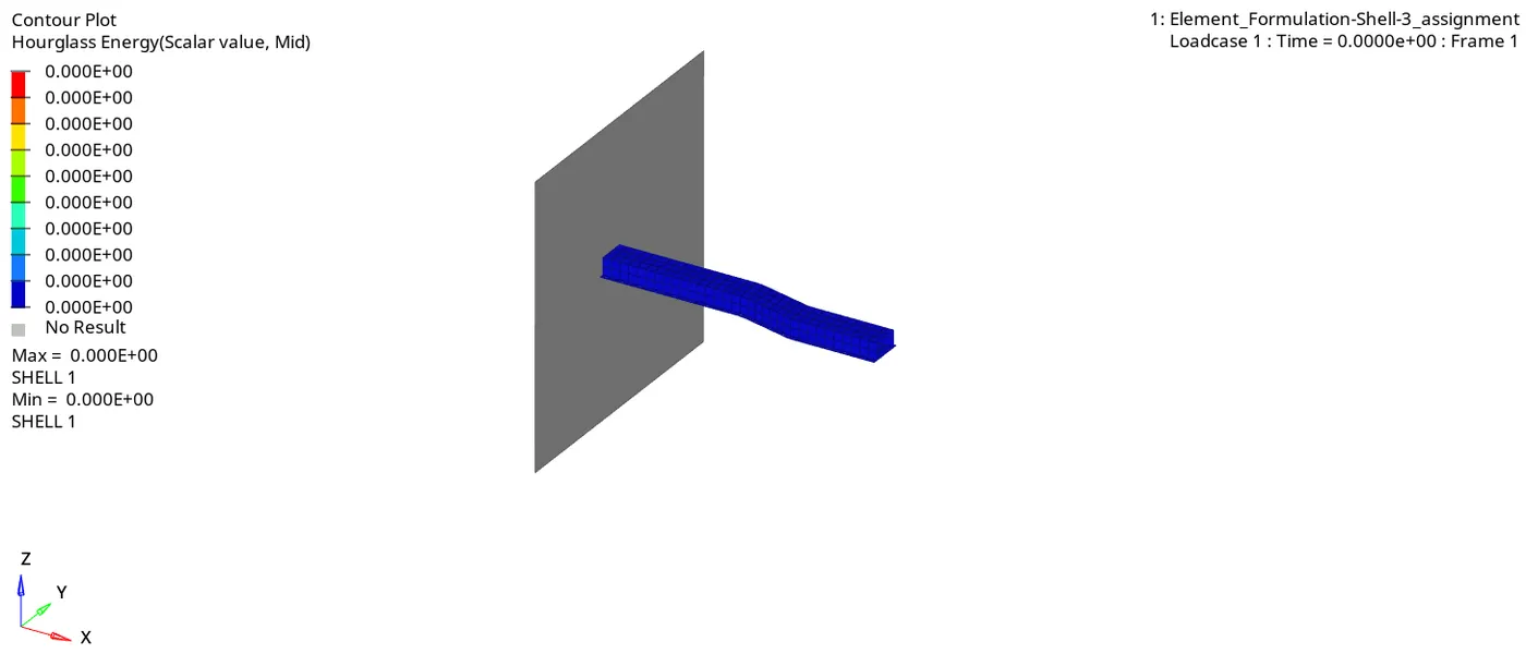
10. Go to Contour - Select Result type to 'Hourglass Energy' - Click Apply.
11. Click play to run the animation.
Report:
1. Case 1 and case 2 graphs.
Case 1
Case 2
2. Case 1 and Case 2 graph plot data of maximum and minimum.
Case 1
| Sr no. | Name | Minimum | Maximum |
| 1 | Internal Energy | 0 | 19285676 |
| 2 | Kinetic Energy | 35680184 | 61314900 |
| 3 | Contact Energy | 0 | 25441.5 |
| 4 | Hourglass Energy | 0 | 6.31597e+06 |
| 5 | Total Energy | 54965860 | 61314900 |
| 6 | Rigid Wall Force (Total Resultant Force) | 20376.6 | 113439 |
Case 2
| Sr no. | Name | Minimum | Maximum |
| 1 | Internal Energy | 0 | 17465234 |
| 2 | Kinetic Energy | 43792244 | 61314900 |
| 3 | Contact Energy | 0 | 7598.86 |
| 4 | Hourglass Energy | 0 | 0 |
| 5 | Total Energy | 61257480 | 61314900 |
| 6 | Rigid Wall Force (Total Resultant Force) | 7655.16 | 114154 |
3. It is seen that Internal energy (max), Kinetic energy (min), Contact (max), Hourglass energy is 0, Total energy(min) and Rigid wall forces (min and max) are changes from case 1.
4. And also there is a change in Energy error in case 1 it is -10.3 % and in case 2 it is -0.1 %.
In case 1 and case 2 Mass error is 0.1659E-03 %.
Energy error: The Energy error is calculated in percentage using the formula:
%Err=100(Ek+Ei+Er_kEk,1+Ei,1+Er_(k,1)+Ewk-Ewk,1-1)">%Err=100(Ek+Ei+Er_kEk,1+Ei,1+Er_(k,1)+Ewk−Ewk,1−1)%���=100(��+��+��_���,1+��,1+��_(�,1)+���-���,1-1)
Where, Ek – Translational kinetic energy at current time
Erk – Rotational kinetic energy at current time
Ei – Internal energy
Ewk – Work of external forces (energy brought to the system)
E,1 – Initial energy (at t = 0)
The Hourglass energy is not considered for the energy balance
The Energy error must be in the range of -15% to +5%.
Mass error : The extra mass is added to the model to reduce the hourglass. The amount of mass added to the original mass of model is called mass error.
5. This changes is happen due to we change the value of Ishell = 24, Ismstr = 2 and in case 2. The value of Ithick, Iplas and N are same on both the cases.
6. And also we change the valvue of Ish3n = 2. But for this simulation if doesn't change the valve is also fine because in the model there are no tria element present in it.
7. We change the valvue of Ishell = 24 (QEPH) and Ismstr = 2.
QEPH is an improved under - integrated 4 node element with 1 integration point on the surface. It uses physical stabilization method to control the hourglass. In this method method hourglass control is good because it treats at material level. Due to which in case 2 the hourglass energy is reduced to 0 as compare to case 1 (it always not go zero). QEPH also increases accuracy due to which we got less energy error and also we got more accurate graphs in case 2.
Ismstr = 2 is used for small strain with full geometrical nonlinearities with possible small formulation activation in RADIOSS Engine.
8. Ithick = 1 - Thickness change is taken in account for accuracy.
9. Iplas = 1 - Interacting plasticity for good accuracy.
10. Hourglass and its correcting method.
Under-integrated elements are very familiar in crash wothiness. In these elements, a reduced number of integration points are used to decrease the computation time. This simplification generates zero energy deformation modes, called Hourglass modes.
There are two correcting methods available
- Peturbation or penalty method: Hourglass control by application of anti-hourglass forces to maintain deformation stability of the element.
- Physical stabilization method: Hourglass control by the correction of internal energy is an analytical way.
For the first method, four formulations are available.
- Type 1 (Default): Only in-plane modes are corrected, valid for shells and solids.
- Type 2: Old formulation no longer recommended.
- Type 3: Plasticity is taken into account in the computation of anti-hourglass forces; in-plane and out-of-plane hourglass modes are corrected; available only for shells.
- Type 4: Link Type 1 with additional higher order terms in the computation of anti-hourglass forces and with out-of-plane hourglass mode correction; available only for shells.
Note: When the material undergoes elastic-plastic behavior, the Type 3 formulation is much more efficient. The hourglass coefficient, hm and hf are recommended to set to 0.1. However the default value hf=0.01 can be used for hr.
The second method is powerful and can be used when the mesh quality is good. The physical stabilization method is incorporated in the following elements.
- QEPH Shell
- HEPH Solid
- HSEPH Solid-Shell
Result and Conclusion:
The results from both cases are compared with each other successfully.
Due to property parameter change in case 2 the accuracy of the case 2 is higher compared to the case 1.