Assignment 3-2D Element Formulation Challenge

OBJECTIVE : To learn about element formulation, all the associated parameters in property module, running the simulations and plot different graphs, check and compare between different simulation results.

PROCEDURE :

• Import the file given in the question.

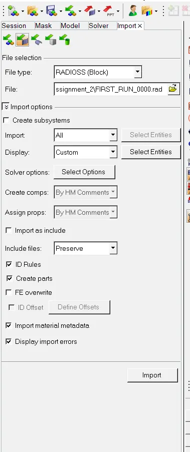
• Change the parameters given in the question. Change run time to 55ms and change the animation steps in between 25 and 60.

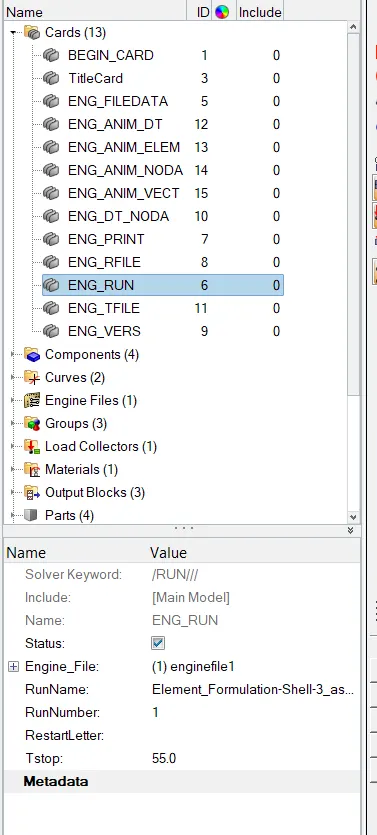
• To change the Run time go to --> model browser --> cards --> ENG_RUN --> Change Tstop value to 55.

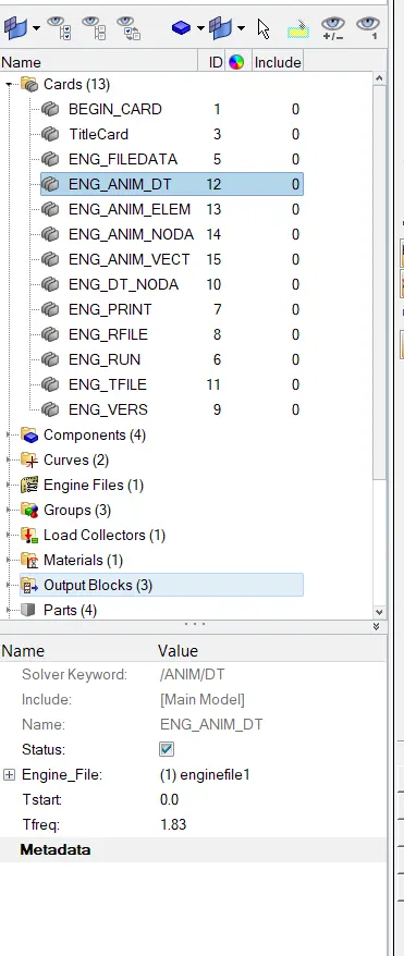
• In the same way, change value of Tfreq value to 1.83 to get no of animation files.
• Run the simulation, for that go to --> Analysis page --> Radioss.

• Select the input file. Select export options as all, run options as analysis and run number as 1.
• In the options box type -nt 4, to increase the computational speed. Save the file and click on radioss button.

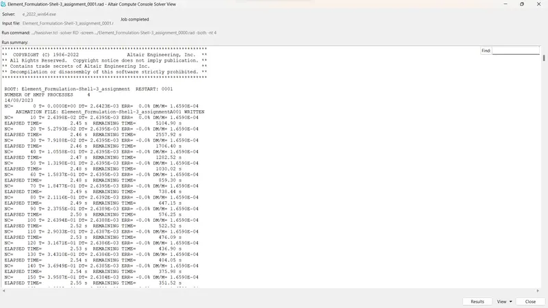
• After running the simulation, we get the result file of radioss. Now, the radioss has solved the model.
• To view the file in hyperview, open the .h3d file which is animation file. Click on view at bottom right side corner of file.
• This will open hyperview window.

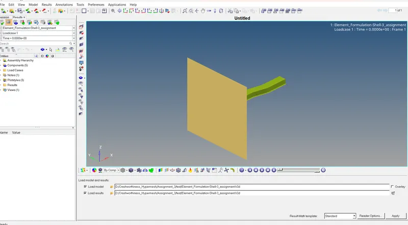
• In hyperview we can run the simulations and check no of parameters such as displacement, velocity, hourglass energy etc.,

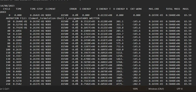
• To check the energy and mass error, find 0001.out file from the folder in which we saved our simulation results, open the file in notepad and check error and mass. error values.
• Energy error should not be more than 1 or 2%. It should be between -15 to -5%. We are satisfied with our results in first case.
• Now, proceed to plotting graphs for rigid wall forces, internal energy, hourglass energy, contact energy and total energy.

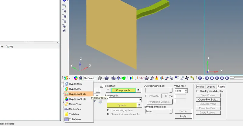
• To plot the graphs, click on drop down button of ribbon, click on HyperGraph 2D.

• In the ribbon section, there is Build Plot option. After clicking on it we get the page as shown in above.
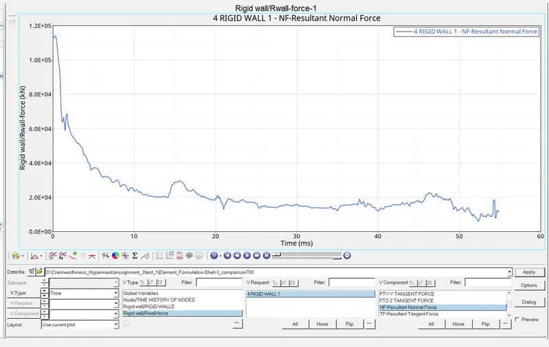
• There select Y-type as Rigid wall force, Y-request as 4RIGID WALL 1 and Y-component as - Resultant Normal Force and click on apply button. Which will plot the Graph as shown in below.

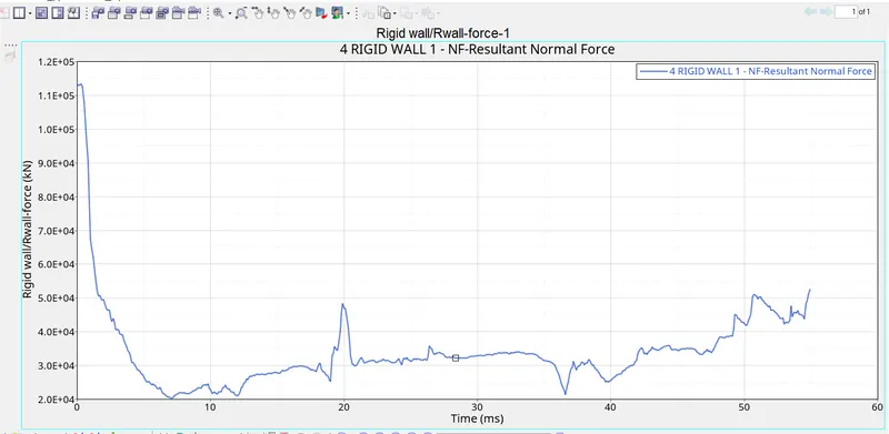
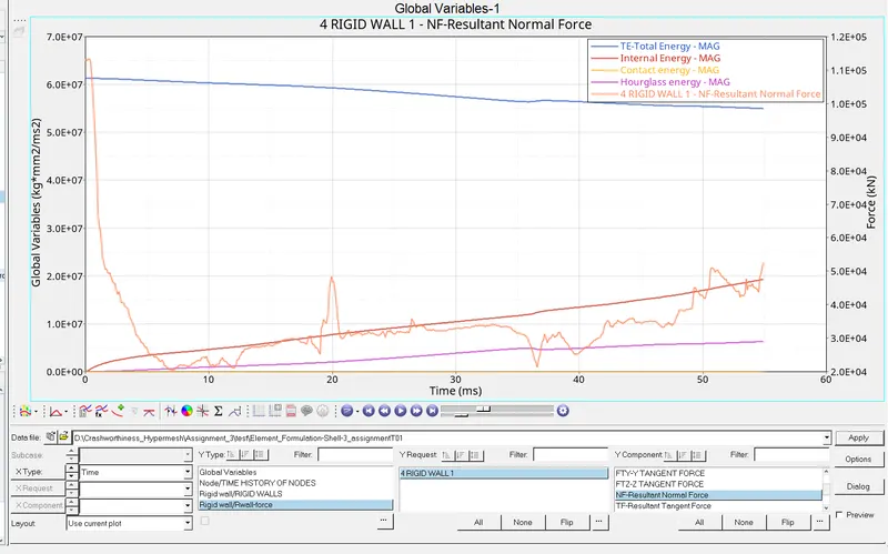
• Here we can see all the graphs together. We will see them each separately later at time of comparison.
• For next model set up change the values from property section and run the simulation again and compare the results.
• For that go to property section of the model.
• Change all the parameters as per given in the question.The parameters are as follows -

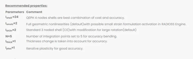
• To change the parameters go to model browser, check the properties section. In the properties section change only shell properties. There are weld properties also do not alter them.

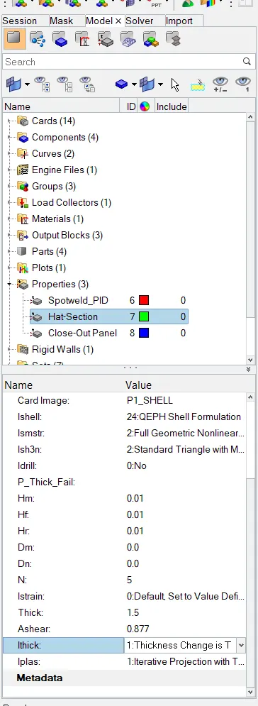
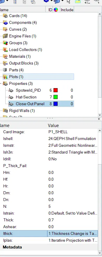
• The parameters as given in the question has been changed. Now proceed to simulate it.
• Go to analysis page, create the new folder and repeat the procedure as we followed for case 1.
• After clicking on radioss we will get the result file. Now plot the graphs for this case as well and compare them with case 1.

Graph 1 :

Rigid wall forces

CASE 1 CASE 2

Graph 2 :

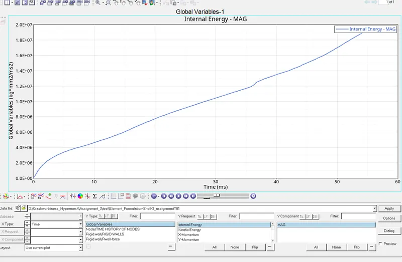
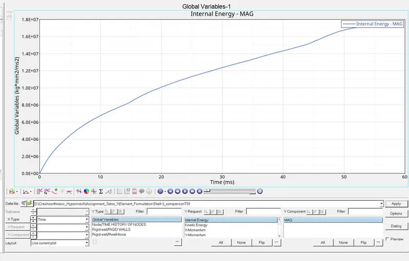
Internal Energy

CASE 1 CASE 2

Graph 3 :

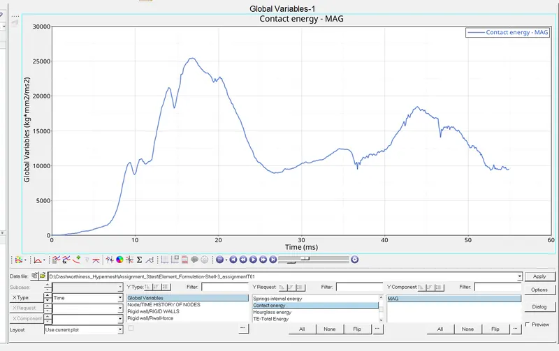
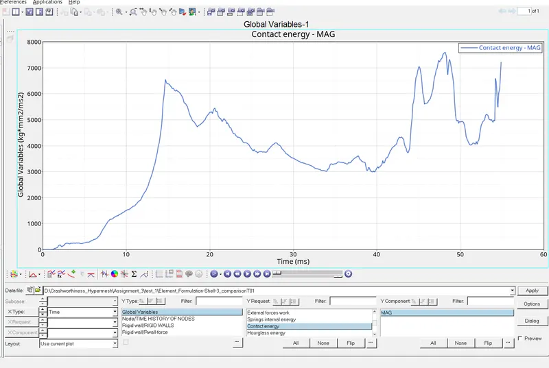
Contact Energy

CASE 1 CASE 2

Graph 4 :

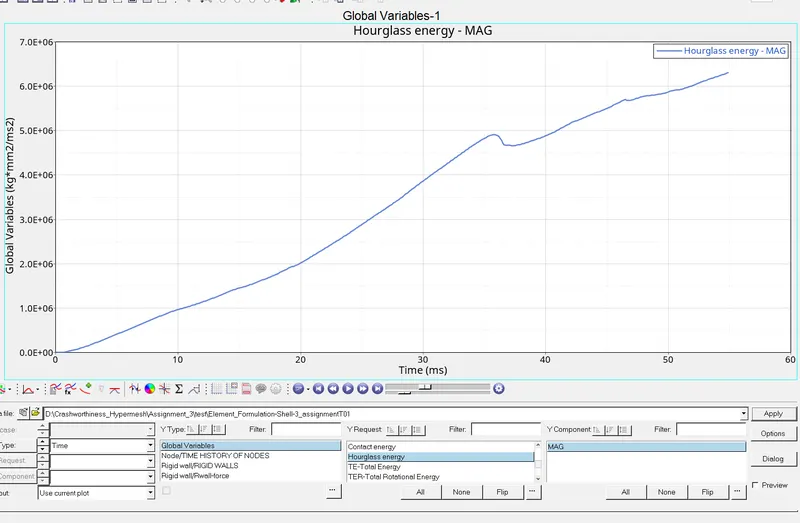
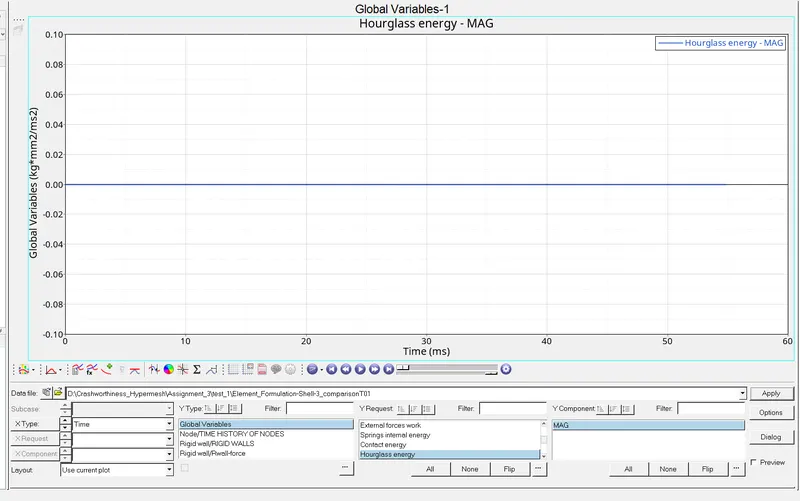
Hourglass Energy

CASE 1 CASE 2

Graph 5 :

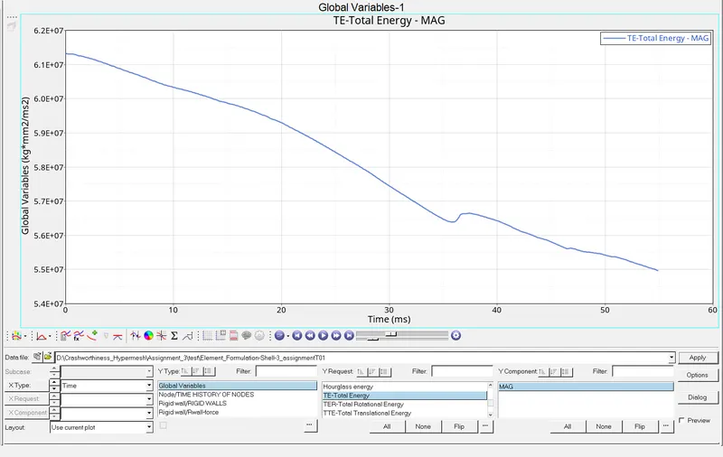
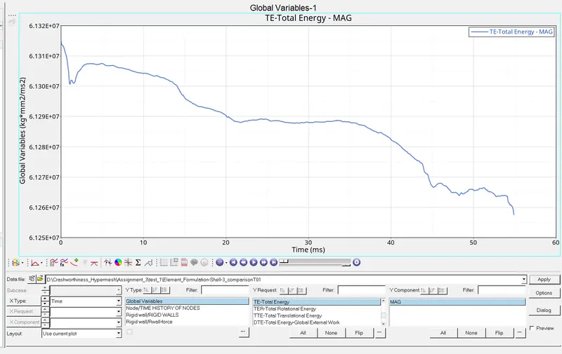
Total Energy

CASE 1 CASE 2

RESULTS :

• We have plotted graphs for internal, contact, hourglass and total energy and rigid wall forces.
• In case 1 we had the parameters given in the question and in case 2 we changed the parameters as given in question.
• After in case 2 we can see that the results are changed a lot.
• For rigid wall forces - the behaviour of curve was different in both the cases. In case 1 the forces were high at start of simulation and they drastically falls as simulation starts. When it reaches the time of 20ms the energy factor was increasing in case 1 while it was decreasing in case 2 for the same time period. In case 1 amount of force at end of simulation is more but in case 2 they are less as compared to case 1;
• For internal energy - the amount of internal energy is more in case 1 as compared to case 2;
• In case of contact energy - the graph in case 1 increases and decreases after but for case 2 it doesn't decrease;
• For Hourglass graph - in case 2 there is no hourglass energy generated, while in case 1 it was present, this change is seen because of type of element that we are using. We changed the Ishell type to 24. Which has improved integration than other elements and low in cost also.

Hourglass Energy :

• Hourglass is a non-physical mode of deformation which occurs in underintegrated elements and produce no stress.
• Hourglass is a type of numerical instability that can occur in some types of elements, such as first order, reduced integration elements.
• This means they have only one integration point and that point can not capture the strain variation happening in the element.
• As a result of this, the element deforms in non-physical way that resembles hourglass shape. This can lead to inaccurate results.
• To avoid hourglassing, we can use different methods. Like - 1 ) Perturbation method; 2 ) Physical stabilization method.

1 ) Perturbation Method ( viscous method )

• The deformation is defined with velocity of nodes.
• When hourglass phenomenon is detected, a force (external) is applied to node to stabilize the deformation.
• This external force will make an element stiffer. This force introduced artificial energy called hourglass energy.

2 ) Stiffness Method

• Hourglass yield depends upon natural yield.
• Excess stiffness is added at material level.
• We can control hourglass even before they arise in model.
• Preferred for lower rate problem i.e., low velocity or low strain rate problems such as crash.