Assignment 3-2D Element Formulation Challenge

COMPARISON OF RESULTS WITH BASE SIMULATION AND IMPROVED SHELL ELEMENT PROPERTIES

 (Crashworthiness Analysis using HyperMesh and Radioss Assignment 3 - 2D Element Formulation Challenge)

AIM

• The aim is to run the simulation on crash beam model with base simulation (default values in hypermesh) and improved shell element properties (recommended properties)

Parameters	value	Description
Ishell	24	QEPH 4 nodes shells are best combination of cost and accuracy
Ismstr	2	Full geometric nonlinearities (default)with possible small strain formulation activation in RADIOSS Engine
Ish3n	2	Standard 3 noded shell (C0) with modification for large rotation(default)
N	5	Number of integration points set to 5 for accuracy bending
Ithick	1	Thickness change is considered for accuracy
Iplas	1	Iterative plasticity for good accuracy.

• Change the elemental properties as mentioned below and check whether the results are acceptable then compare the results with the base simulation.
• Study the output of both the simulation by plotting Rigid wall forces and Energies like internal energy, Hourglass energy, Contact energy and Total energy.

Objective:

1. Using the crash beam file from the previous assignment, change the run time to 55 ms.

2. Change the number of animation steps during simulation to a minimum of 25 and a maximum of 60.

3. Run the base simulation without any modification to element properties.

4. At the end of the simulation, do the energy error and mass error checks and determine whether the results would be acceptable.

5. If acceptable, Plot rigid wall forces, internal energy, hourglass energy, contact energy, the total energy of the simulations.

6. Change all the shell elements properties to recommended properties, save this as separate, rad files and run the simulation.

7. Follow steps 5 and 6.

8. Create a brief report comparing all the results from steps 5 and 6 for both simulations.

9.Comment whether there is any change in the results and why there is any change in the result.

What is Hourglass?

• It is weird mode of deformation that occurs in under integrated shell elements where no stresses are produced. As stresses are not produced, it reduces the accuracy and true response of the structure. This leads to inaccurate strain and displacement results with unrealistic deformations. 

  

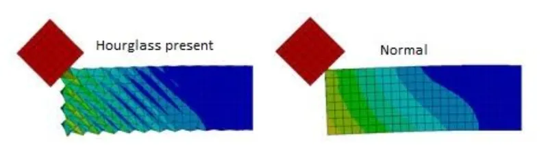
  When do we say that hourglass is produced?

  • In an under-integrated element, displacements and forces exist for each node of the element. If the summation of all these forces and displacements provides zero stress and strain on the integration point of the element, then that element fails to calculate the stiffness for the mode of deformation. Due to no stiffness calculation, the deformation happens in a very weird manner. This is when we call, the element has entered into hourglass.

  How is hourglass controlled?

  • As mentioned before, the hourglass occurs only at the under integrated shell elements. To avoid hourglass, we go with reduced integration elements. We saw two types of reduced integration shell elements: Ishell=1,2,3,4 and Ishell=24, The control of hourglass also changes on the type of shell elements used. Ishell=1,2,3,4 (Q4) employs perturbation method for controlling hourglass. Ishell=24 (QEPH) employs a physical stabilization method for controlling hourglass.
  • Perturbation Method: In Ishell=1,2,3,4, the hour glass deformation is detected with motion of the nodes. If it is detected, an apposing force is applied on the node to stabilize the deformation. The amount of force inputted is based on the model’s material applied like young’s modulus, yield stress and plastic tangent. This apposing force produces an artificial energy called hourglass energy. One disadvantage is that Q4 elements fails in case of large rotation and elastic loading-unloading cycles.
  • Physical Stabilization: In Ishell-24, shell elements control the hourglass from the material level. Here, the hourglass loading stiffness and hourglass yield depends on that model’s material properties like natural tangent modulus and natural yield respectively. By this way, the hourglass is stabilized QEPH elements. Advantage over Q4 is that it works perfectly well at all kinds of loading-unloading cases.

  PROCEDURE:

  Objective1: This first question requires us to change the run time to 55 ms. For that, we first need to import the solver deck file in question to RADIOSS

  • Go to File >> Import >> Solver Deck. This brings up the import menu. Here, we can select the file we need to import. This file is called starter input deckfile, which is the file that ends with '0000.rad'.\

                                                   

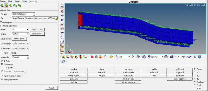
                                                                                                                     Imported RAD file

  • Now, change the run time to 55 ms (as required). To do that, we need to go to the solver tab >> engine_keywords >> run >> eng_run, we can now edit properties of ENG_RUN in the small window as shown below.

                                                                                                      

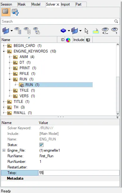
                                                                                                               Changing Animation Steps

    Objective3: Run the base simulation without any modification to element properties

                                                                                                            

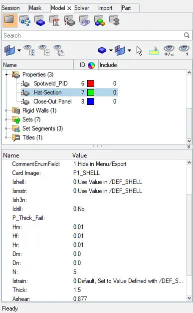
                                                                                                              Properties for base simulation

    • For this, we can go to the Analysis >> RADIOSS.
    • In the next section, we are given the option to save the file before running it in the solver. We can go ahead and give it a different name from the base file to avoid confusion. Clicking 'save as'. It creates a new folder and saves all the output files.

                                               

                                                                                                  Saving analysis with new name

    • It is recommended to be written as "-nt 4" as shown in the image below. This means assigning the task to 4 cores in the system, to perform the simulation faster. It depends upon the process of our computer (it has a quad-core processor, then it should be taken as 4, If the system has an octa-core processor, then it is taken as 8). And "nt" means "number of threads". Then click on "Radioss", in order to run the simulation.

                                           

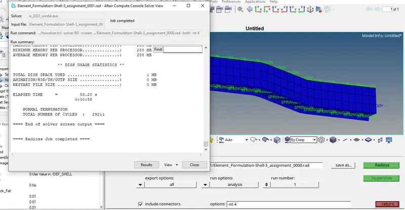
                                                                                                       Analysis is done

                                               

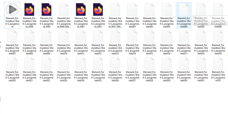
                                                                                                       Files Created After Analysis for default values

• The simulation is complete, now we just need to visualize it. For that, we need to switch to the Hyperview utility.
• This can be done by clicking the client selector option in the toolbar or can be activated from view > toolbars > hyperworks > client selector. In that menu, we can select Hyperview to switch to it.

                                                  

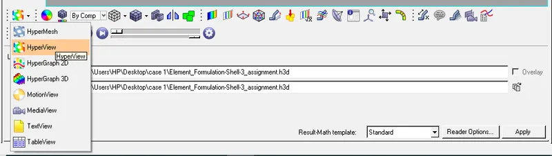
                                                                                                                Switching to Hyperview

• After accessing Hyperview, we should input the simulation file. For this, use h3d file that was generated when RADIOSS processed the starter file. It is generated in the files swhich are shown in the picture above. After selecting it, we can click 'apply'

                                                 

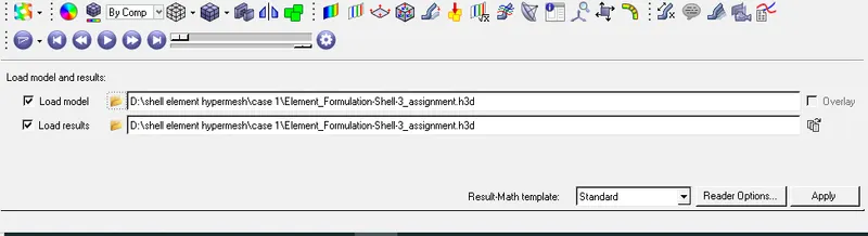
                                                                                     Opening h3d file which was created by RADIOSS simulation

• Doing so generates the simulation animation. We can change what is being represented by selecting the 'contour' option in the toolbar

• Objective4: At the end of the simulation, do the energy error and mass error checks and determine whether the results would be acceptable.

  • The next step is to check the obtained values for energy error, internal energy, total energy, mass error from the engine output file (00001.out).

                                           

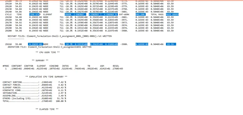
                                                                                           Engine output file for default values

  • In the same file, when it is scrolled down to last, the maximum values are seen as shown in the image below. From the figure, the obtained maximum values are energy error: -10.3%, Internal energy: 0.1932E+08 gm^2/s^2, Kinetic energy: 0.3563E+08 gm^2/s^2.
  • The acceptable tolerance for energy error is -15% to +5% .The closer to 0 it is, the better.

   

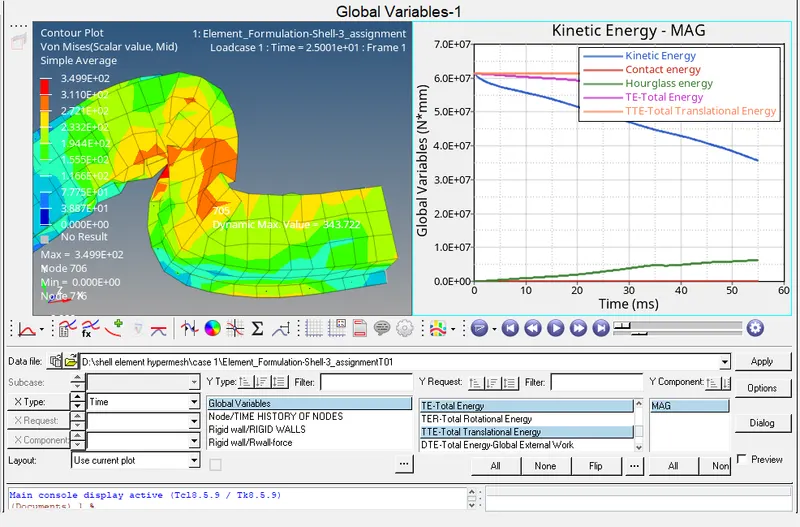
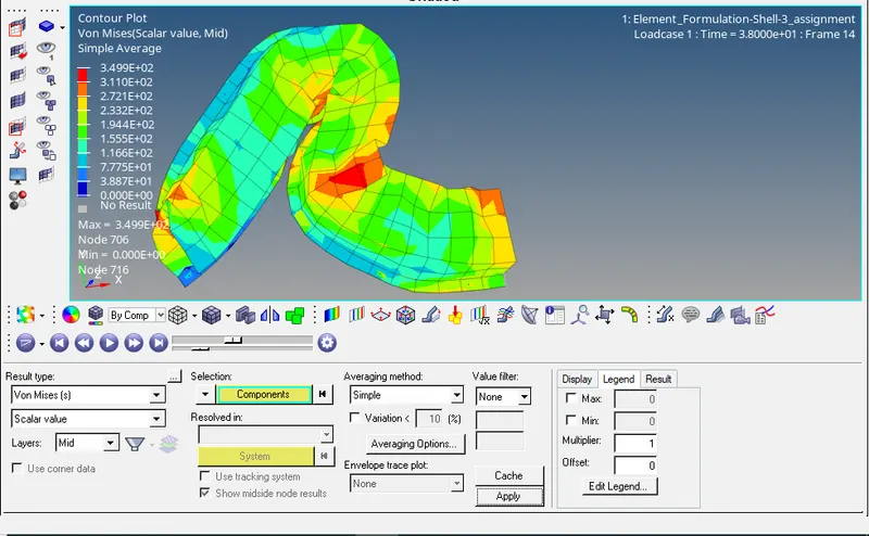
• Objective 5:  If acceptable, Plot rigid wall forces, internal energy, hourglass energy, contact energy, the total energy of the simulations

  • With the energy and mass errors deemed acceptable, we can go ahead and plot the graphs. For this, open Hypergraph 2D. We can switch to it using the same client selector option in the toolbar.

                                                                                                   Opening Hypergraph 2D

  • In the Hypergraph section, we need input a file. For this, we will be using the result file generated by the RADIOSS solver which is in 'T01 file'. This file is available in the same directory as the starter, engine, and animation files. The file name ends with 'T01'.
  • Select the required options as shown below to plot all the graphs

                                             

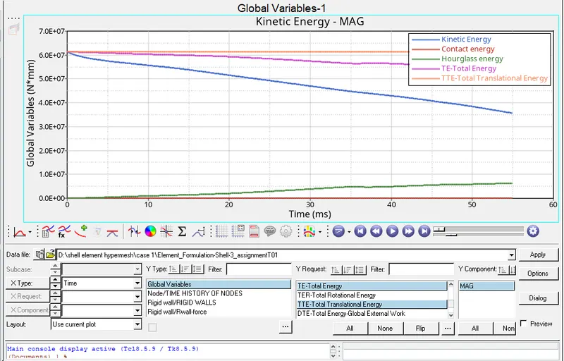
                                                                                            Graphs formed by default properties

  Kinetic energy (KE): We know that the formula for kinetic energy is 1÷2mv^2. Since the velocity is applied to the component, there will be a high velocity at the beginning. This velocity decreases with respect to the time, due to the deformation within the rail component. So, the kinetic energy is directly proportional to the velocity. That is the reason why, the kinetic energy drops gradually, as shown in the graph below.

Internal Energy: In the beginning, there is no displacement within the component, that’s why the internal energy starts from zero(origin). when it is subject to acceleration there will be a displacement. As the displacement increases, the internal energy increases, that’s why there is a raise internal energy curve, as shown in the graph below.

Hourglass Energy: As the recommended properties are not specified in this case, there will be a deformation of elements with respect to the strain is not recorded. Which depicts that, the elements undergo an hourglass effect. And there will be no physical stabilization. So, to balance the energy, artificial energy is required. That is hourglass energy. So, there is a lot of hourglass energy needed. So, the hourglass energy starts from the origin and goes on increasing, as shown in the graph below

Total Energy: As the hourglass energy increases, more amount of energy is not recorded. As a result, total energy is decreased as the graph progresses.

• Now, Create a new plot and generate the graph for rigid wall forces using Rigid Wall/Rwall Force - 4 RIGID WALL 1 - total resultant force as shown below.

                                   

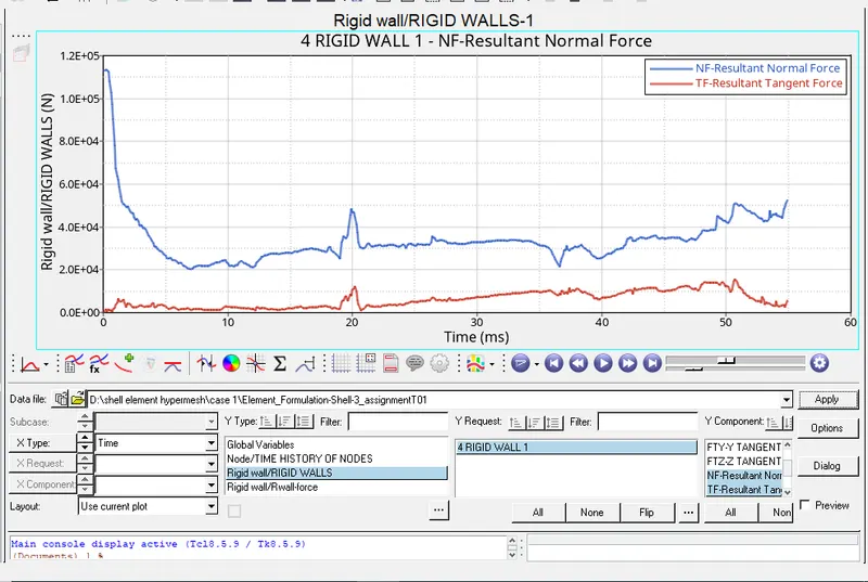
                                                                                Total resultant force by Default properties

Objective 6: Change all the shell elements properties to recommended properties, save this as separate, rad files, and run the simulation.

• For this question, we are to carry out a simulation for a new case with the recommended shell element properties. We can repeat the process of importing the original solver deck file and change the values of Run time = 55ms, Tstart= 0 ms &  Tfreq = 1.375 ms in the solver tab. (Tfreq=Run time/Number of step)
•                                                      
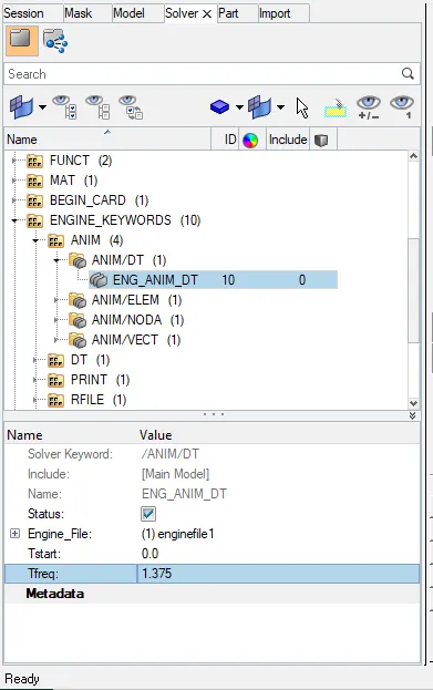
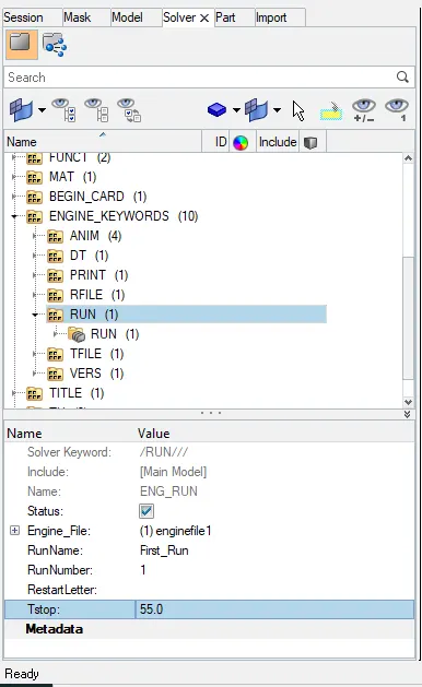
• Now, edit the properties as shown below.                                                               

                                                                     

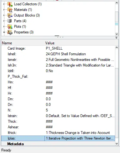
                                                                        Recommended Properties

• Now run the simulation again and store all the output files in different folder.

                                      

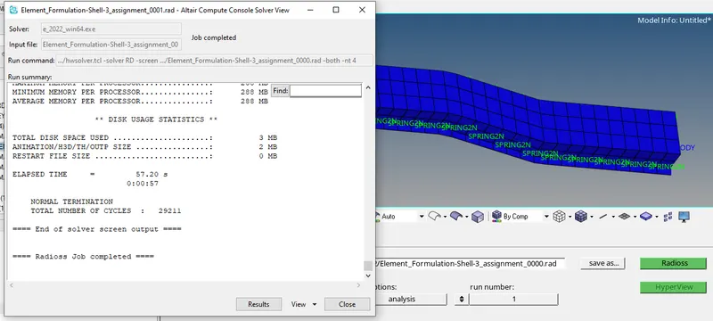
•                                                               Analysis is done for recommended values

                                         

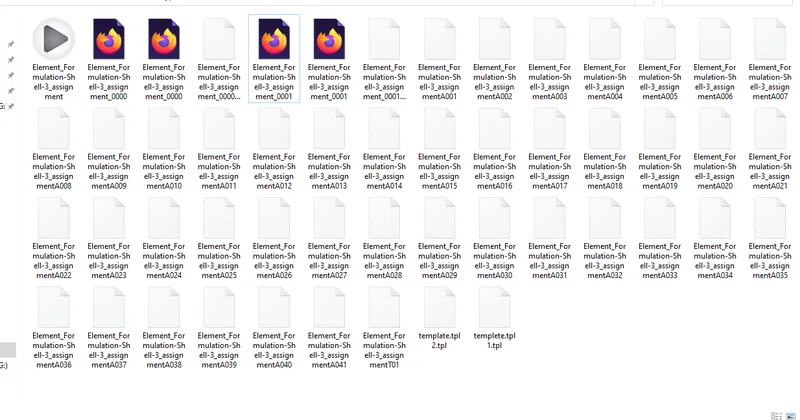
                                                                                      Files Created After Analysis for recommended values

  • After that, we can switch to Hyperview to generate the simulation. Like last time, we need to pick the h3d file of this case and click apply.

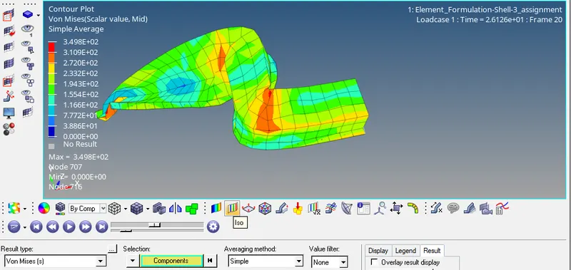
      Animation shows Von Mises stress contour for recommended values

   

  Objective 7: Follow objectives 5 and 6

  • The next step is to check the obtained values for energy error, internal energy, total energy, mass error from the engine output file (00001.out).

                                       

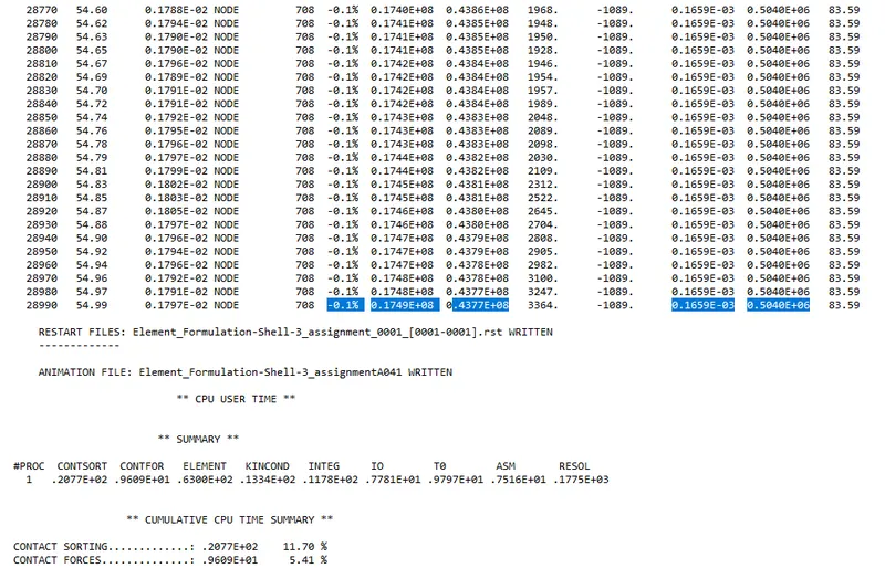
  • As we can see, there is a drastic reduction in energy error, as was evident in the more natural-looking simulation. Earlier the hourglass energy is -10.3% now it was reduced to -0.1%, which is almost zero.
  • Hourglass energy: As the deformation starts increasing the hourglass energy gradually increases because of the Default property i.e., 0- DEF SHELL has a single integration point and it has no stabilized properties, hourglass increases. 
  • Whereas in the Recommended property i.e., QEPH-4 the hourglass energy is zero because the property of the element has improved with 4 noded integration points and it has physical hourglass stabilization property. Thus it avoids the hourglass completely in this case.
  • Now we can generate the graphs by switching to Hypergraph and selecting this simulation's T01 file. Firstly, the energy graph:

                                         

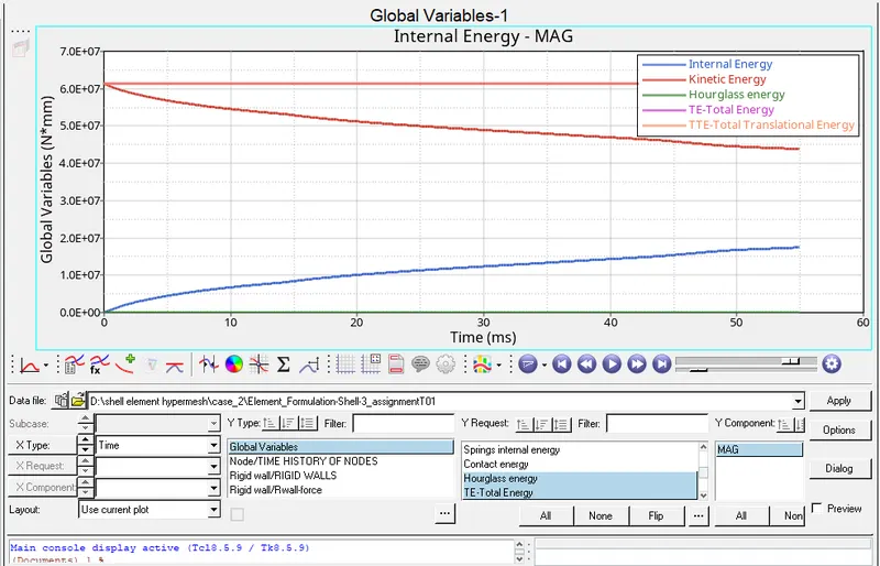
                                                                                 Graphs formed by Recommended properties

                                          

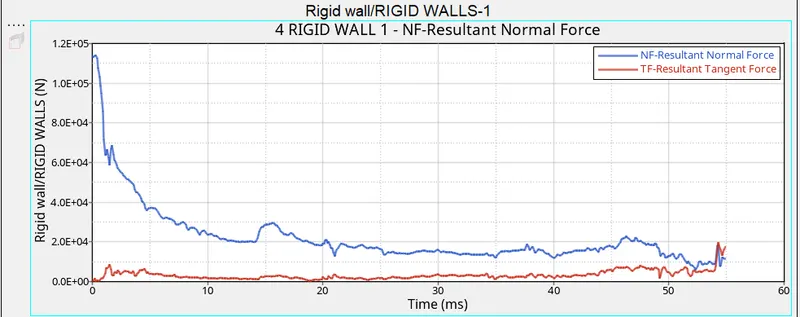
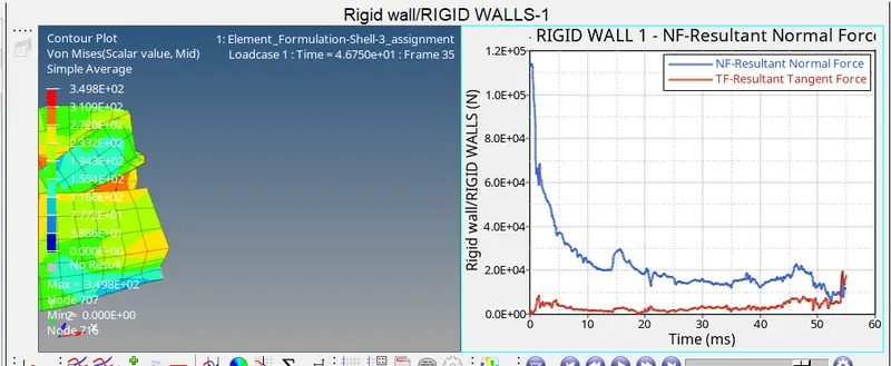
                                                                                      Total resultant force by Recommended properties

  Objective 8 & 9: Create a report comparing both simulations and comment on results obtained

  • We can open plots of both cases simultaneously as shown below. This makes comparison easy

                                           

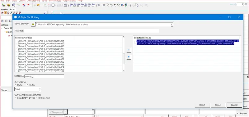
                                                                                    Opening two T01 files at same time in Hypergraph 2D

Opening two T01 files at same time in Hypergraph 2D

                                               

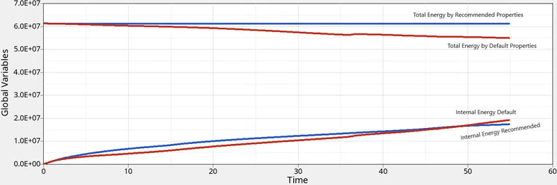
                                                                                                 Comparing results obtained in both cases

• The obvious difference in both simulations is the reduction in hourglass energy. The introduction of QEPH shell formulation (Ishell= 24) in the second case, provides an artificial stiffness to the shell elements and helps counter hourglass formation.
• Therefore, the simulation with RECOMMENDED properties is looking more natural compared to the default simulation
• I have created a table below which compares both the simulations

Attribute	Default Property	Recommended Property
Energy Error	-10.3% which is acceptable	-0.1% A good number since its almost 0.
Internal Energy	0.1932E+08	0.1749E+08
Kinatic Energy	0.3563E+08	0.4377E+08
Hourglass Energy	Hourglass energy increase over time, since they have no physical stabilization in defoult properties.	Hourglass energy is zero, since they have all the recommended properties, physical stabilization is done before hourglass energy generation.
Total Energy	As the hourglass energy increase, more amount of energy is not recorded. As a result, total energy is decrease as graph progress.	As there are no hourglass energy lost, the curve remains constant.

                                       

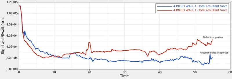
                                                                                                Comparison graphs of resultant forces

• The more realistic simulation also resulted in a different resultant force graph that represents the collision events more realistically.
• The formation of a kink at around 20 ms causes a sudden spike in case 1, whereas in the second simulation, as the QEPH shell formulation is used, there is no sudden spike as the elements are deformed in a much better manner. Understandably, there is a large force at the beginning, which happens at contact, and is the same in both cases.

Learning Outcomes

• Learned about different Property settings used for better simulation results in HYPERMESH RADIOSS user profile
• Carried out simulations for both default and recommended values in Hyperview
• Plotted all the required graphs using Hypergraph 2D

Conclusion:

All the required objectives are fulfilled. Simulations are carried out using both default and Recommended properties. Comparing both cases, we can easily say there is difference in the values of hourglass energy, internal energy, and rigid wall forces. Recommended settings helped reduced hourglass drastically due to the introduction of the physical stabilization method that is deployed by QEPH elements Deformation occurred under recommended settings is looking more practical.