Assignment 3-2D Element Formulation Challenge

1. Objective:

• To run the base simulation with the default values took by the software( i.e., With out changing the properties), which is taken as case 1.
• To run the new simulation after assigning the properties, which is taken as case 2.
• To plot the various graphs, which depicts the internal energy, hourglass energy, contact energy & total energy and compare with the both results.

2. Software used: Altair Hyperworks Desktop 2022

3.User profile: Radioss

4. Pre-requisites:

Element formulation:

There are so many elements that we use in radioss to get the desired results. And these elements are categorized by the element formulation technique, which consists of the same elements but varies with respect to some parameters such as type of integration with in the element, cost etc. Based on this element formulation, we can specify the type of elements to be used in our simulation. These are explained below.

In general, there are 3 types of elements. Based on dimensions. They are:

• 1D elements: Which includes Springs,Trusses, Beams.
• 2D elements: Which includes shell elements like quads(4-noded), Trias(3-noded).
• 3D elements: Which includes solid elements such as Tetra, Hexa elements.

1D elements:

Truss:

• A truss is a 2 noded element, Which possess the tensile or compression behaviors only.
• It is compatible with elastic & elasto-plastic materials.
• It's property is defined by cross-sectional area.
• This property appears in the solver as PROP/ TRUSS.

Spring:

• A spring is a type of 1D element which undergoes only for tension or compression behavior.
• The applications of this element are linear elastic, Non-linear elasto-plastic materials.
• This property appears in the solver as PROP/SPRING.

Beam:

• A beam is defined by 3 nodes, in which it's orientation is defined by the 3rd node.
• It's property is defined by cross-sectional area & inertia's.
• This property appears in the solver as PROP/BEAM.

2D elements:

2D elements are also known as " shell elements". As mentioned above, there are 2D elements. They are: quad & tria elements

2D Element formulation:-

Before going to the 2D shell element formulation, An important parameter should be discussed. Which is named as "Hourglass".

Hourglass:

"Hourglass is a deformation, that is noticed when an element is deformed due to the applied load. But the strain energy due to this deformation is not recorded for that element". It is also known as "Zero energy deformation modes" where an element is seen deformed.

• It indicates the instability.
• It is also said to be as, non-physical modes of deformation, that occur in reduced or under integrated elements & produces no stress.
• Usually, it can be seen in the post-processing stage, where the elements will have zig-zag formation.

The elements with before & after experiencing the hourglass effect is shown in below figures.

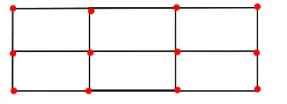
Before experiencingHorglass effect

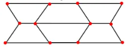
After experiencing hourglass effect

Methods to control the formulation of hourglassing:

There are two methods to control the houglass effect. They are:

1. Perturbation method(Viscous method)
2. Physical stabilization method (stiffness method)

Perturbation method(Viscous method):-

• This method is generally used for the elements with Ishell: 1,2,3,4 or Q4 elements.
• The process how this method work is: When the hourglass deformation occurs---> There will be some damping applied, which is stabilizes the deformation, that results in controlling the speed of deformation.
• But this damping opposes only the velocity, But not the force. So, the force is introduced, which results in adding some stiffness to the elements. This stiffness helps in controlling the hourglass.
• The force is applied externally, by some other means. But not from FEA nature. This force constitutes some an energy called"Hourglass energy", Which is an artificial enenrgy(neither Kinetic or inetrnal energies). It is a loss of both energy types.
• If the hourglass enenrgy is added along with the kinetic energy & Internal energy, A balance system is obtained.
• Recommended for high velocity or high strain rate problems. Example: Involving high explosives.
• Huge amount of hourglass energy is generated.

Stiffness method:-

• In this method, the stiffness is getting added right from the material level. This will have a large effect on our component.
• It is recommended for less velocity problems.
• used for QEPH elements.
• Less amount of hourglass energy is needed. Because, it is going to be controlled before it arrises.

The 2D element formulation is shown in below fig.

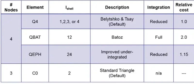
As shown in above figure, there are 3 types of element formulations for a quad elements(which is 4-noded). These are explained below.

Q4 element:

• It is a under(or) reduced- integrated element. Because, it has only 1 integration point for an element.
• It is represented in the radioss solver by an entity named " Ishell(1,2,3,4)".
• Usually Ishell:1, Ishell:4 elements are used, when no more velocities are to be found.
• By default, the solver takes as Ishell:1.
• As it has only 1 integration point, the time required to solve the problem with this type of element is relatively less.
• The cost required to solve this type of elements reletively low.
• But there will be no accuracy in the results.

QBAT element:

• It is a fully-integrated element, Which means it comprises of 4 integrated points. Each point near to the each node.
• It is represented in the radioss solver by an entity named "Ishell: 12".
• Because of this 4 gaussian integration points, there will be no Hourglass deformation.
• Using this element is not economical. But the achieved results are more accurate than the remaining Ishell elements of quads.

QEPH element:

• It is improved under-integrated element with the physical hourglass stabilization with in itself.
• It is represented in the radioss solver by an entity named "Ishell:24".
• This type of element is mostly used recently. Because of its best compomise between the cost, quality& accuracy in results.
• It is widely used in the automotive industries.

CO element:

• It is a standard co-rotational triangle, with modification for large rotations.
• Usually, it helps in representing the tria elements with the entity named "Ish3n:2".
• It consists of 1 integration point.
• No hourglass deformation.
• Low CPU cost.
• Results may not be accurate.

Difference between reduced integration & fully integrated schemes:

Reduced integration	Full integration
It will have only 1 inegration point.	It will have 4 integration points.
Decreases the computation time, when compared to the full integration method.	It will take more time for computation. Because of more integration points.
The obtained results are less accurate.	The obtained results are accurate, when compared to reduced integration.
Hourglass can not be controlled.	Hourglass can be controlled.

Key parameters in /PROP/SHELL:-

There are 6 main parameters for shell elements, They are:

Ishell:-To select the element formulation for 4-noded shell elements.

Ish3n:-To select the element formulation for 3-noded shell elements.

N:- To choose the number of integration points through the thickness

Ismstr:- To specify whether the strain formulation is small or large.

Iplas:- To choose method for the calculation of post-yield strain.

Ithick:- To determine if the thickness is constant under load or if the element thins.

The significance of these parameters and the recomended values are explained below.

Ishell:

It is same as explained about the Q4,QBAT,QEPH elements explained above.

Recommended element: QEPH(Ishell: 24)

Reason: This element is a improved under-integration with the physical hourglass stabilization with in itself. Better accuracy and cost effective, when compared to Q4 elements.

Ish3n:

It is same as explained about the CO element explained above.

Recommended element: CO(Ish3n:2)

Reason: In order to compensate with the larger rotations. ANd it is taken by

N:

In this parameter, the number of integration points to be taken with respect to the thickness of element is choosed.

N	Number of Integration points through the thickness
0	Global integration method (Default).
1≤">≤≤N≥">≥≥10	Number of integration points from 0 to 10.

In radioss, N is accepted upto 10.

Recommended value: N=5

Reason: In such cases, it will have 1 integration point on the surface of the shell element & 2 integration points on the either side of the shell element.

Ismstr:

By this parameter, the stain with which the elements are subjected to, is decided(Small or large).

Ismstr	Shell strain formulation
1	Small strain from time=0
2	Large strain with full geometric non linearities (default)

Small strain:-

• It is suitable for the small deformation problems.
• The Strain computed is based on initial element shape.

Large strain:-

• It is suitable for the large displacements and strains.
• The strain computed is based on the current element shape with the derivative of the shape function.

Recomended: Ismstr:2

Reason: For achieving the accurate results, the deformations took place in the elements should be taken in to account instantly.

Iplas:

Before going to discuss about this parameter, another concept named "Stress computation" should be known.

The stress is obtained in this process: Forces at the nodes---> Acceleration----> Displacement---> strains---> stress.

With these computed stress values, the von-misses stress is computed and compared to the yield stress of the material. The von-misses stress takes care of normal stresses in two directions ansd shear stresses.

If the von misses stress is <"><< the yield stress of the material, then the computed stress is used to compute the internal force of the elements. This internal forces calculates the next time step.

If the von-misses stress is>">>> the yield stress of the material, it depicts that the plastic behavior is reached. Then the Iplas come in to picture. It acts as a switch for the sover to indicate that, the given material is subjected to plastic behavior.

Iplas	Shell plane stress plasticity flag
1	Iterative projection with 3 N iterations
2	Radial return (Default)

Recommended value: Iplas:1

Reason: For getting accurate results, the solver should understand the plastic behavior is stareted and the results with that behavior is also required. But it will take time when compared to the Iplas:2.

Ithick:

Ithick	Thickness change
1	Thickness change is taken in to account
2	Thickness is constant

Recomended value: Ithick:1

Reason: For getting the accurate results, whatever the change in the thickness is happened while deformation is taking place, should be taken in to account.

So finally, to have the accurate results. The values for the those parameters should be as mentioned below:

Ishell=24

Ish3n=2

Ismstr=2

N=5

Iplas=1

Ithick=1

5. Procedure:

Case -1(Without assigning the recommended parameters in the property):-

Initially after opening the altair hyperworks desktop software, the user profile should be selected. And the user profile to be selected is "Radioss" as shown in fig 5.1. Because, for performing the analysis.

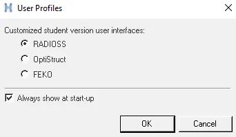
fig: 5.1

The next step is to import the given rad file(starter file). This is done by clicking on import, selecting the solver deck in it. After selecting the solver deck, a pop-up appears as shown in fig 5.2. In which the given rad file is browsed and by clicking on import, the model with respect to that rad file is imported.

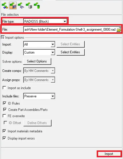
fig 5.2

After importing the model, it appears as shown in fig 5.3.

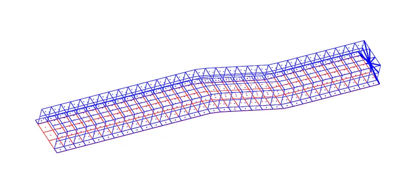
fig 5.3

As the model is in wireframe mode to view it properly, an option named "shaded elements with mesh lines" is enbled. After enabling it, the given model appears as shown in fig 5.4.

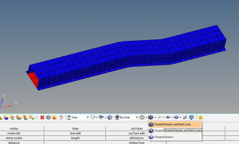
fig 5.4

The next step is to assign the time step value in the card named "ENG_RUN" as shown in fig 5.5. As mentioned in the question, the run time or time step is 55 ms. This value is entered in the parameter named "Tstop".

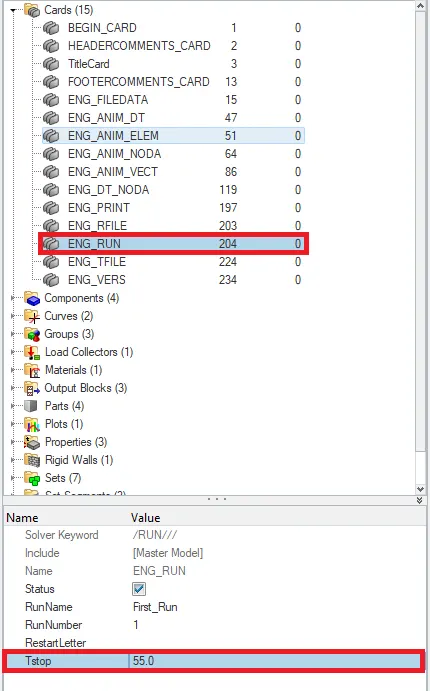
fig 5.5

The next step is to select the number of animation steps required. As mentioned in the question, number of animation steps can be beween 25 to 60. In this challenge, the number of animation steps selected is 50.

Now to calculate the Tfrequency for run time as 55 ms with respect to the 50 animation steps.

Formula used: Tfreq = Time step ÷">÷÷Number of animation steps

= 55÷">÷÷50

= 1.1

Therfore, the Tfreq is 1.1.

This value is entered in the parameter named "Tfreq" in the card named "ENG_ANIM_DT" as shown in fig 5.6.

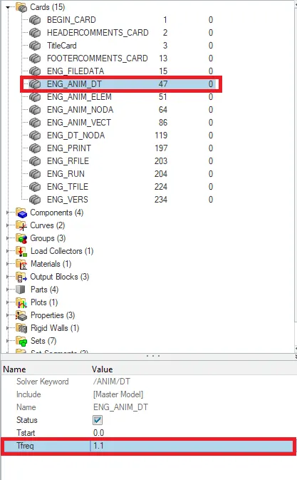
fig 5.6

These values are entered just to perform the simulation.

As in this case, the results are obtained without assigning any properties to the given components. The parameters in property card are taken the default values as shown in fig 5.7.

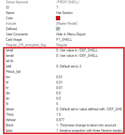
fig 5.7

The next step is to run the simulation. For doing that, the "radioss" option is used in the "Analysis" panel as shown in fig 5.8.

fig 5.8

After entering in to the radioss panel, Initally the file should be saved in some folder using "save as", and in the options it is recommended to be written as "-nt 4" as shown in fig 5.9. Which means assigning the task to 4 cores in the system, to perform the simulation faster. It depends up on the process of our computer( It it has a quad core processor, then it should be taken as 4. If the system has a octa core processor, then it is taken as 8). And "nt" means "number of threads". Then click on "Radioss", in order to run the simulation.

fig 5.9

After completing the simulation, the radioss solver sends a pop-up as shown in fig 5.10. Which indicates the simulation is completed.

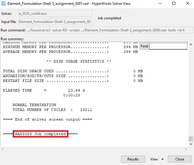
fig 5.10

The next step is to verify the assigned values such as Tfreq, Tstop in the engine rad file (00001.rad) in notepad++. The changed values appears in that file as shown in fig 5.11.

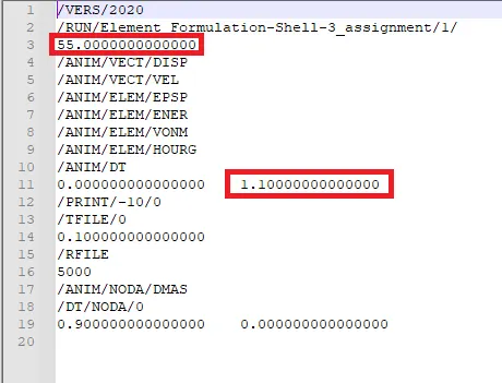
fig 5.11

The next step is to verify the required number of animation files are obtained in the file location that is specified at the beginning. As the specified number of animation steps are 50. The obtained number of animation steps are 51. These are shown in fig 5.12.

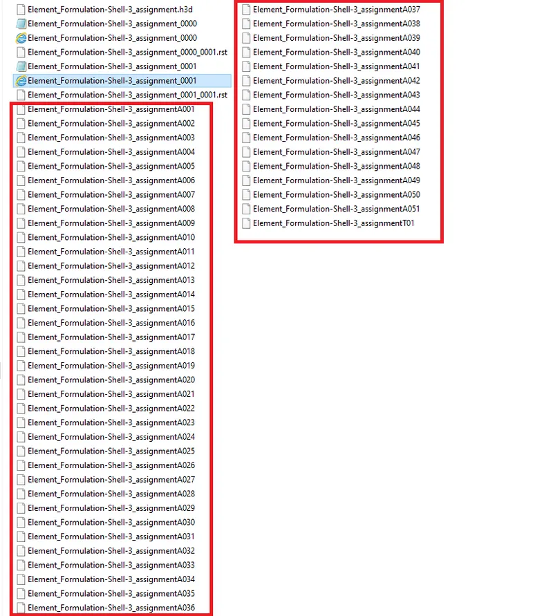
fig 5.12

The next step is to check the obtained values for energy error, internal energy, total energy, mass error from engine output file(00001.out). These values appears as shown in fig 5.13.

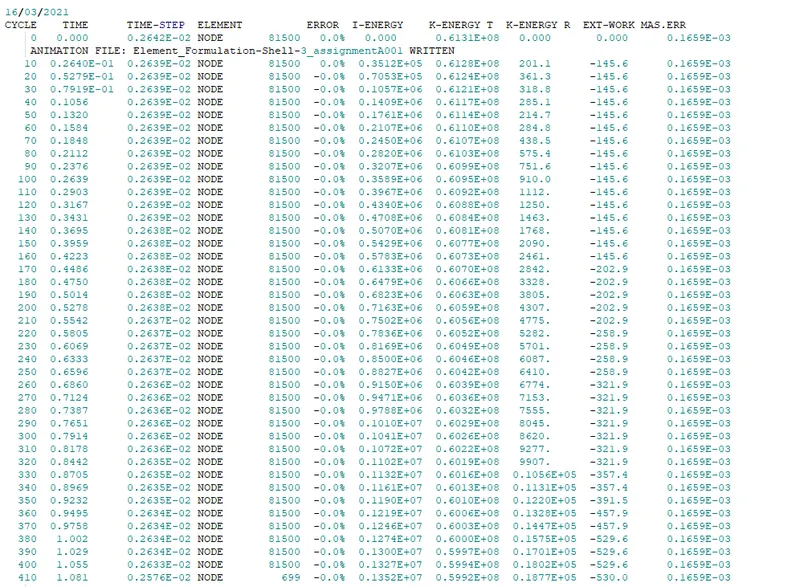
fig 5.13

In the same file, when it is scrolled down to last, the maximum values are seen as shown in fig 5.14. From the figure, the obtained maximum values are energy error: -10.3%, Internal energy: 0.1928E+08 gm^2/s^2, Kinetic energy: 0.3569E+08 gm^2/s^2.

Note: The acceptable tolerance for energy error is -15% to +5%.

fig 5.14

Then click on "results" as shown in fig 5.10, inorder to have a new window. After opening a new window, it automatically switches to hyperview from hypermesh. It shows to import the h3d file and click on Apply as shown in fig 5.15. In order to view the simulation.

fig 5.15

After importing the h3d file, it appears as shown in fig 5.16.

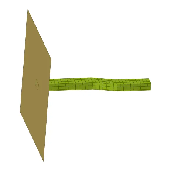
fig 5.16

Then, the next step is to enable the contour. This is done by selecting the highlighted symbol as shown in fig 5.17.

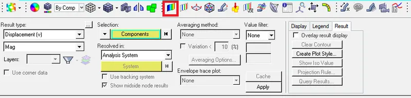
fig 5.17

The next step is to select the various parameters such as the way to view as von-misses, selecting the components, selecting the averaging method, Then click on apply at the end as shown in fig 5.18

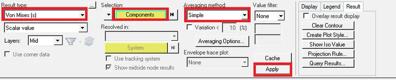
fig 5.18

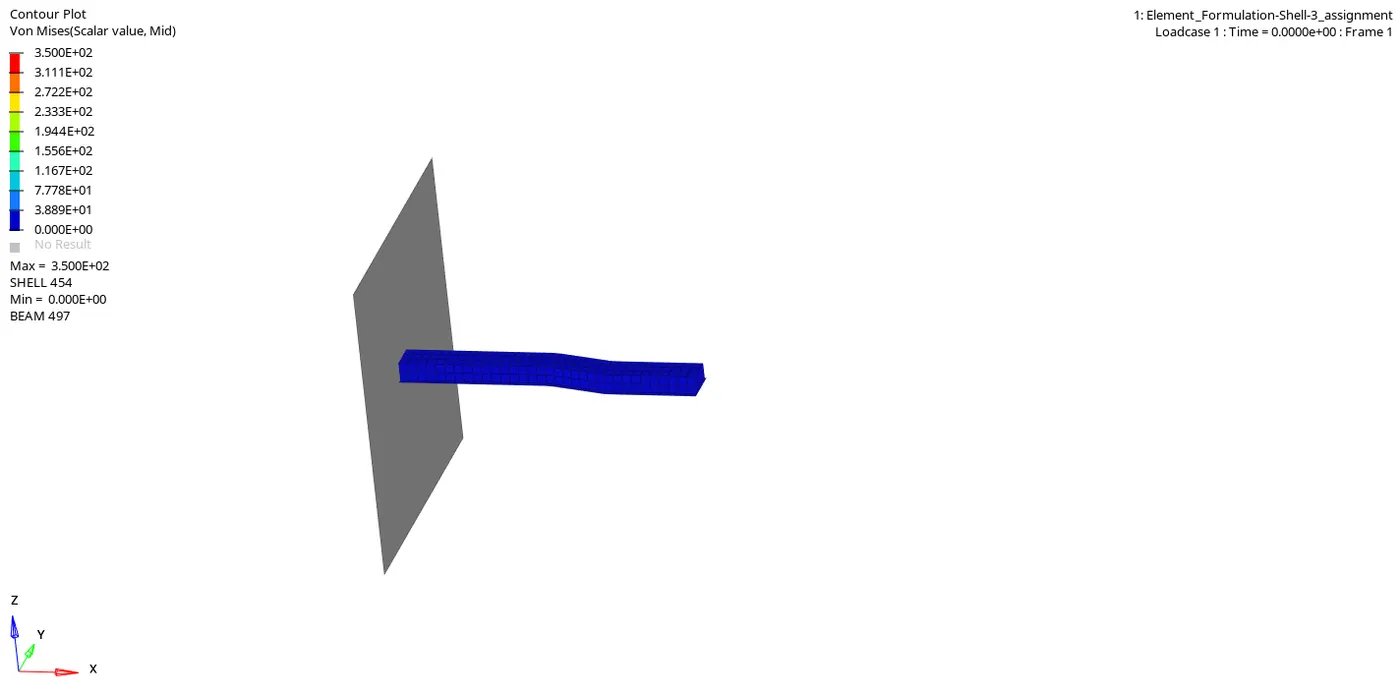
After applying that, run the simulation. The simulation appears as shown in the below animation.

The next step is post- processing, This is done by obtaining the various graphs for the above simulation. Inorder to view what is happening with in the component(Rail). This is done by switching to Hypergraph 2D as shown in fig 5.19.

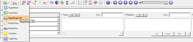
fig 5.19

After switching to the hypergraph 2D, the first graph to be plotted is choosed as to obtain the rigid wall forces. So, the various parameters such as the parameter to be on Y-axis(Rigid wall force), the component to be on Y-axis(Total resultant force) which indicates the term be in the graph are choosed, and then click on "Apply" as shown in fig 5.20.

fig 5.20

The obtained rigid wall force graph appears as shown in fig 5.21. The reason for the rigid wall force is dropping from top is, Initially the rigid wall force acts with in the rail component. At that time, the rigid wall force will be maximum, which is indicated as the starting point of the curve. Slowly that force is observed by the adjacent elements, which leads to the decrease of force(results in falling of curve). And this curve again raises up because the rail component is getting contact with the rigid wall. In this way, rigid wall foces fluctuates..

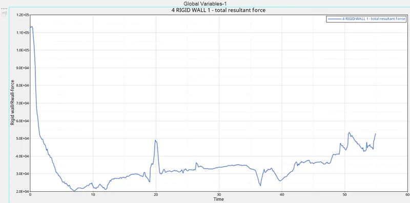
fig 5.21

The next step is to plot the graph that indicates some various important parameters such as Internal energy, Kinetictic energy, Total energy, Hourglass enenrgy. Those parameters are selected and applied from the Hypergraph 2D panel as shown in fig 5.22.

fig 5.22

The obtained graph appears as shown in fig 5.23. The reasons for behavior of the obtained curves are explained below:

Kinetic energy (KE):

We know that, the formula for kinetic energy is 1÷">÷÷mv^2

Since the velocity is applied on the component, there will be high velocity at the beginning. This velocity decreases with respect to the time, due to the deformation with in the rail component.

So, the kinetic energy is directly proportional to the velocity. That is the reason why, the kinetic energy drops gradually, as shown in fig 5.23.

Internal energy(U):

We know that, the formula for internal energy is obtained from first law of thermodynamics. Which depicts the change in internal energy is equal to the difference of the heat transfer in to the system(Q) and work(W) done by the system.

Mathematically, U = Q - W

let us neglect the heat transfer here, because the heat transfer is not calculated by the sover(Because, Thermal analysis is not done). Now, Work done (W) is the product of force and displacement. The internal energy depends up on the displacement mush here. At the beginning there is no displacement with in the component, That's why the internal energy starts from zero(origin). when it is subject to the acceleration there will be a displacement. As the displacement increases, the internal energy increases, That's why therer is a raise internal energy curve, as shown in fig 5.23.

Hourglass energy:

As the recommended properties are not specified in this case, There will be an deformation of elements with respect to the strain is not recorded. Which depicts that, the elements undergo hourglass effect. And there will be no physical stabilizaion. So to balance the energy, an artificial energy is required. That is hourglass enenrgy. So, there is a lot of hourglass energy needed. So, the hourglass energy stars from origin and goes on increasing, as shown in fig 5.23.

Total energy:

We know that, Total energy is the sum of kinetic energy and potential energy. As there is no potential energy plotted here, the kinetic energy is taken in to account. The total energy is directly proportional to kinetic energy. As the kinetic energy decreases, the total energy also decreases, as shown in fig 5.23.

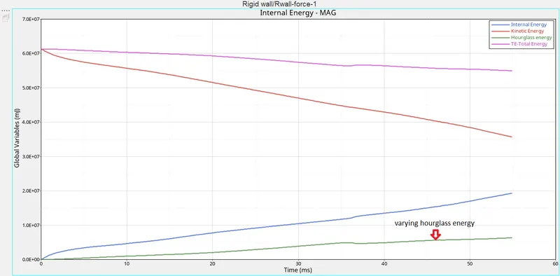
fig 5.23

The next graph to be plotted is contact energy. In the hyperaph 2D panel, all parameters with respect to the contact energy are entered and applied as shown in fig 5.24.

fig 5.24

The obtained graph for contact energy appears as shown in fig 5.25. The reason for the behavior of the curve to be like as fig 5.25 is, Initially there will be no contact between the rail component and rigid wall. And also there is no contact with in the component, That's why the curve starts from origin. And gradually, it reaches to the peak because of more contact witht in the elements of the component due to the deformation.And it drops down as shown in fig 5.25. It raises slowly again to some extent because, there will be a contact between the component and the rigid wall. And due to this contact between the wall and the contact takes place again and again, There will be a regulation in the curve as shown in the fig 5.25.

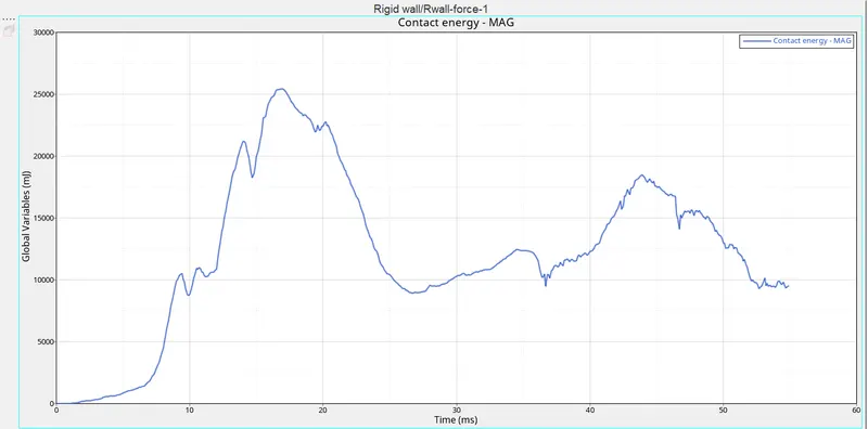
fig 5.25

Case 2(With assigning the recommended parameters in the property):-

In this case, the properties which are recommneded in the question are entered. The procedure is same as in case-1 till entering the parameters in the property cards. After entering the recommended properties, the property card appears as shown in fig 5.26.

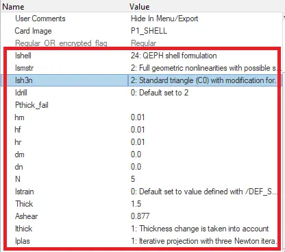
fig 5.26

Note: Save this new file in another location. Inorder to have the entire animation files, engine output files seperately with respect to the first case. To compare the results.

After doing the analysis through the radioss option in the analysis panel, the verification is done to check the required number of animation files are obtained or not. Then the engine output file is opened to view the various parameters such as kinetic energy, Internal energy, energy error etc. as shown in fig 5.27. These values are much less when compared to the obtained values in case-1. Which depicts the improvement.

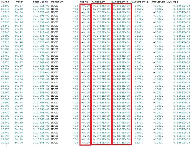
fig 5.27

The next step is to run the simulation. For that a new window is required. So, in the tool bar there will be a option to split the windows. In this case the number of windows splitted is 6, as shown in fig 5.28. Then in the new window, by using hyperview panel, the h3d file is opened. The opened h3d file appears in the second window, as shown in fig 5.28

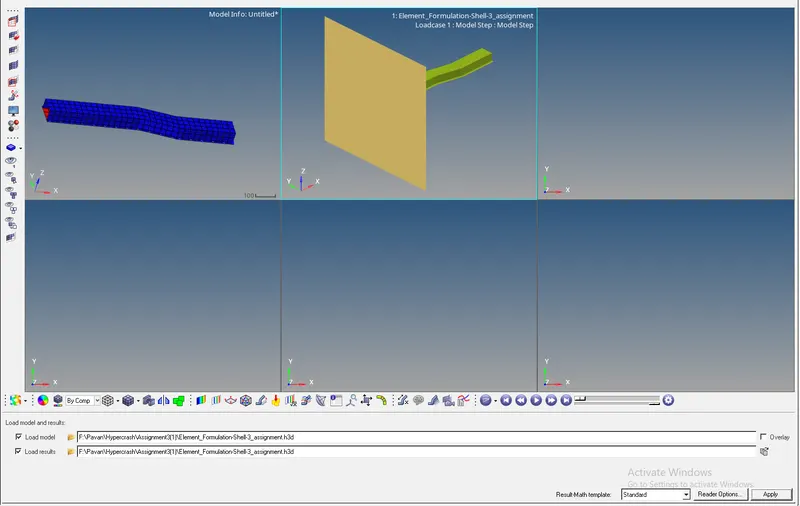
fig 5.28

The obtained simulation, with respect to von-misses view appears as shown in the animation below.

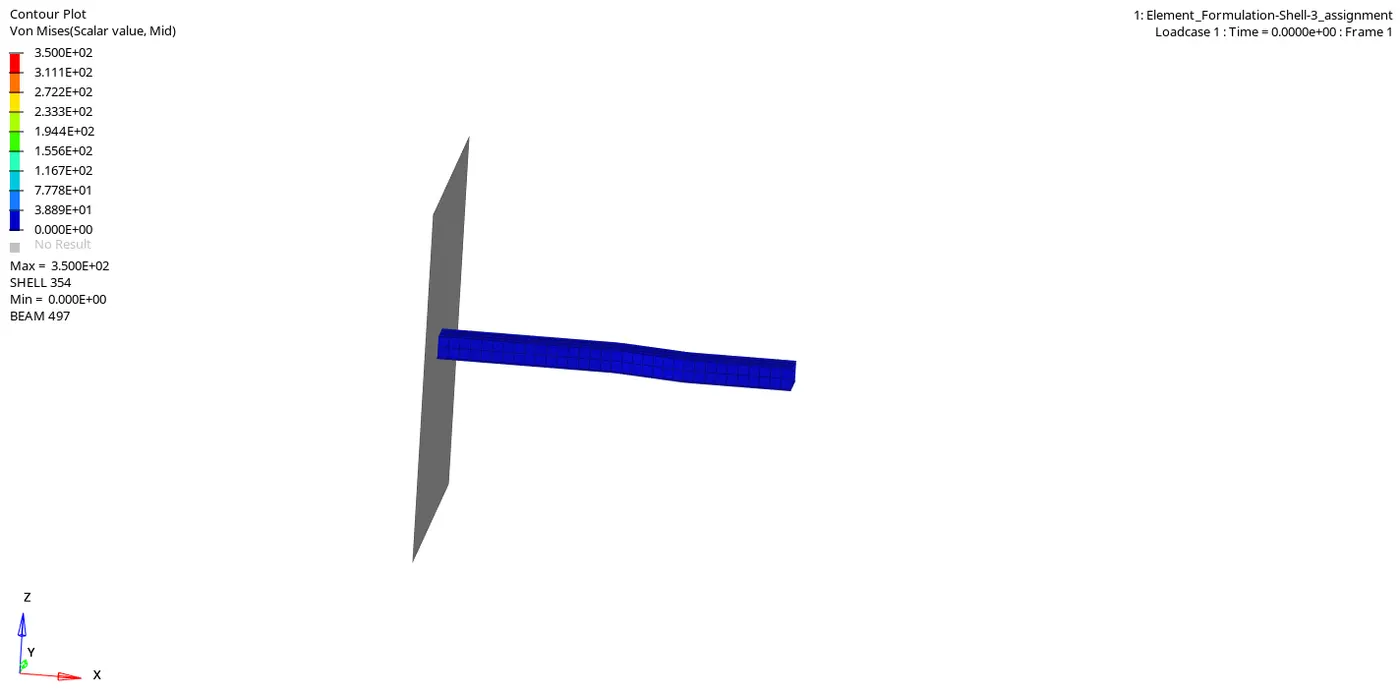
The next step is post processing, In this process various graphs are obtained. Inorder to see the changes in the result with respect to the case-1. The process of obtaining the graphs is same as in case-1.

The obtained rigid wall force graph appears as shown in fig 5.29. The graph appears as similar to that of case-1. And there is some improvement in the graph.

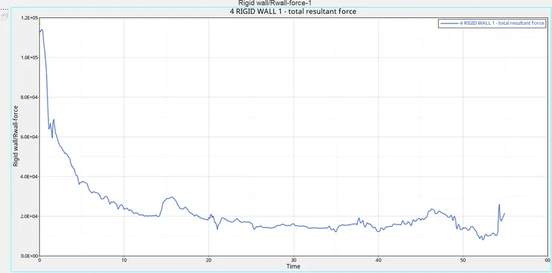
fig 5.29

The next graph consists of parameters such as Internal energy, kinetic energy, Total energy, Hourglass energy as shown in fig 5.30. The graph seems to be some what similar in the aspects of kinetic energy, internal energy. Byt there will be a small raise in total energy, and the hourglass energy is constant as shown in fig 5.30.

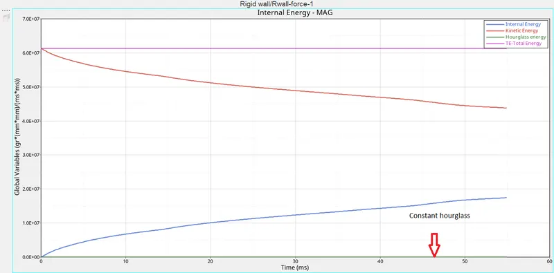
fig 5.30

The final graph to be plotted in this case is contact energy graph, the obtained contact energy graph appears as shown in fig 5.31. It is similar to that of in case-1.

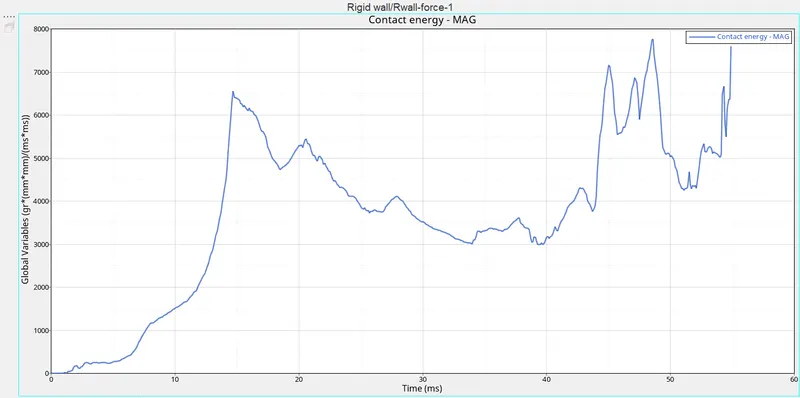
fig 5.31

Note: The same system of units should be used in all cases.

Comparision between the results of case-1 & case-2:-

Basis for comparison	Case-1	Case-2
Obtained maximum energy error	-10.3%	-0.1%
Obtained maximum kinetic energy	0.3563E+08	0.4376E+08
Obtained maximum Internal energy	0.1932E+08	0.1750E+08
Hourglass energy	Varying houglass energy	Constant hourglass energy
Reason for hourglass energy	The elements doesn't have physical stabilization(Due to the default values in the property cards).	The elements have physical stabilization(Due to the assigning of recommended values in the prorperty cards).
Requirement of hourglass energy	it requires hourglass energy to the energy balance.	No hourglass energy is required to balance the energy.
Results	The results are less accurate	The results are accurate

6. Conclusion:

• Therefore, runned the base simulation and new simulation.
• Compared the results obtained in the both cases.
• Finally, I will recomend the same values for the parameters of property cards, to achieve the better results.

7. Learning outcomes:

While performing this challenge, the following aspects can be learned:

• Performing the simulation(Solving- Ding analysis).
• Obtaining the graphs(Post-processing) with respect to that simulations.
• Comparing the obtained values of various parameters such as kinetic energy, Internal energy, Hourglass energy, Total energy etc.
• Recommending the parameters for the properties to achieve good results.