Assignment 3-2D Element Formulation Challenge

Objective: 

To learn about 2D element formulation by running simulation in default and adding properties afterwards and comparing the results.

Cad model image:

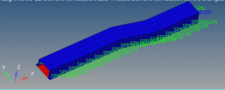
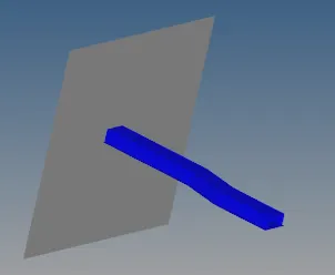
Procedure:

Case 1

• 1st we import the .rad file, then we change the time of simulation to 55ms as given in the question. (ENGINE RUN card)
• 2nd step is to calculate the frequency i.e. to put the timestep, as we are given the choice to select the timestep between 25 to 60, I have taken 40.
• So we calculate timestep freq by dividing run time by number of step i.e. 55/40=1.375. (ANIM DT card)
• Then with default properties we run the simulation in Analysis- Radioss.

• Here, we put the file location where we want the simulation file, then we tick the box of include collectors and in option we should put -nt 4. This is important part as -nt 4 is speeds up the simulation speed.
• Then click Radioss.

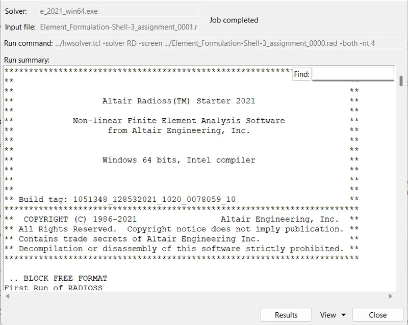
• This will appear, then go to view and click on output file.
• In the output file, we will get the energy errors and mass errors in the most bottom part.

• Here, the energy error is -10.3% and mass error is 0.1659E-03.
• After clicking radioss, we will get result folder in the file location we put it, there we will find h3d file and the T01 file which are the important files that will help us in simulation and to plot graphs.

Case 2

• Now, we should put the properties given in the questions in 2nd case and put the value of time step and run time similar.
• And repeat all the steps we did in case one to get the energy error and mass error.

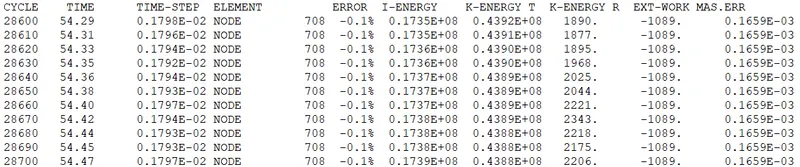
• Comparing the result with case 1 we can see that the energy error is reduced to -0.1%, while the mass error remains the same. 
• For case 2, we should save results in different folder.

Now, for both the cases we have to plot graphs for rigid wall forces, internal energy, hourglass energy, contact energy, total energy of the simulations.

• To plot the graphs best way is to divide the screen into 4 parts so that we can have our model in one part(hypermesh), the simulation in 2nd(Hyperview) and global variable graphs in 3rd(Hypergraph) and rigid wall forces in the 4th part(Hypergraph).

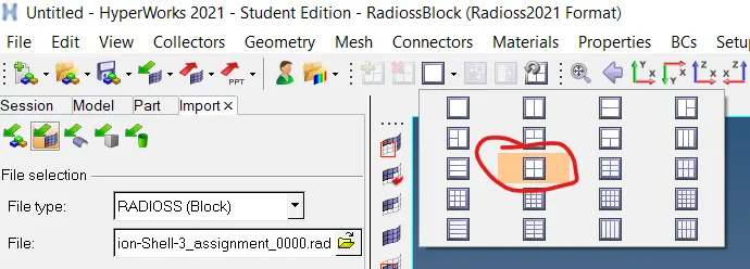
• Now, click on the part to go there like if we want to go on 4th part click on 4th part and we can also maximize and minimize with the help of option highlighted in red in the image below.

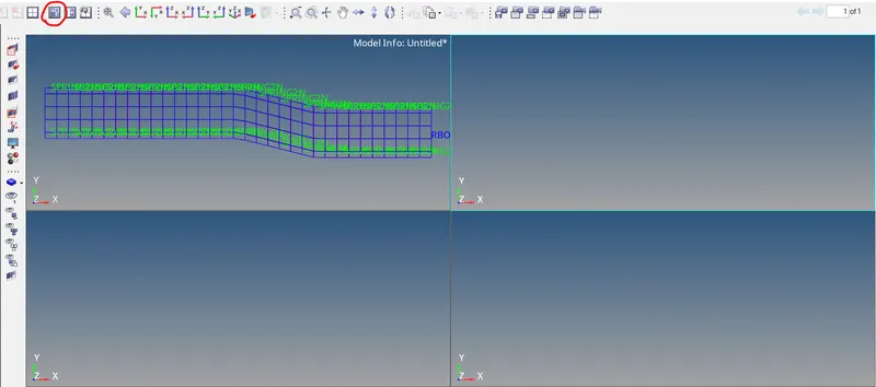
• Now we can see in the image above that the 2nd part is highlighted at the edges because 2nd part is selected, likewise we can select 3rd and 4th.
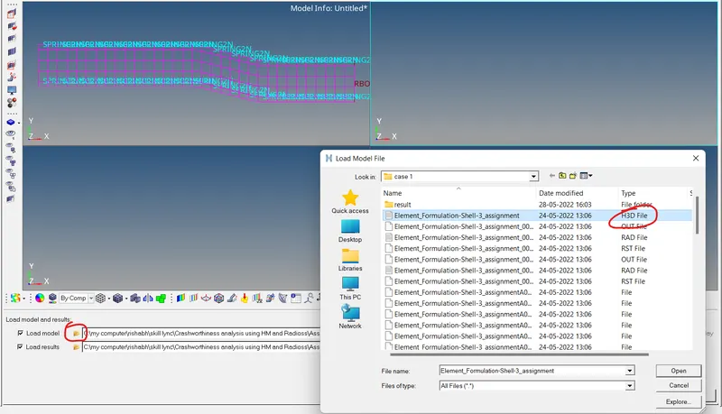
• Now in hyperview i.e 2nd part we should import the h3d file that would give us the physical simulation of how the bracket reacts when it is crushed in the rigid wall.

 

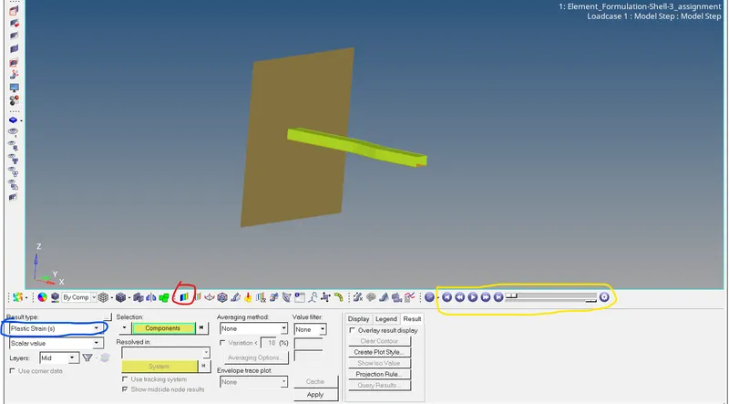
• The red option is contours, yellow is simulation play, pause, speed, etc and blue is the contour, we select the contour, then component, then averaging method if we need it and then click apply.
• If we want to clear the contour there is an option for clear contour also and then we can apply new contour.

• For graphs, we should select the 3rd part of screen and go to hypergraph 2D.

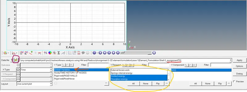
• Here, voilet is for importing file i.e. T01 file.
• Orange shows the global varialbes example internal energy, kinetic energy, contact energy, hourglass energy and total energy.
• Then click apply.
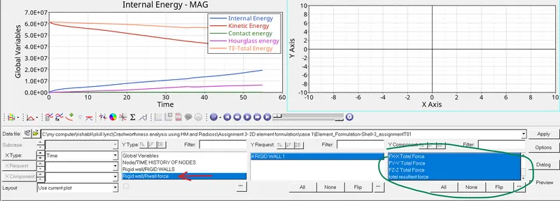
• Similarly for rigid wall forces we should select Rwall forces instead of global variables and select the energies we have to plot. 

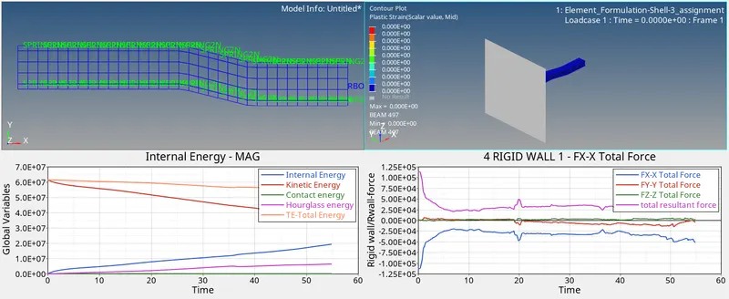
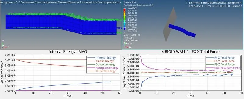
• Similarly, we should do for case 2 and compare the results.

Result and final model:

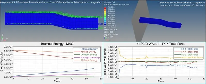
Case 1: In default properties-

Case 2: After applying properties-

Result observations made by graphs-

• In 1st case we can see that the hourglass energy is increasing, while in 2nd case the hourglass energy is zero.
• The Rwall forces are also more uniform than the 1st case.
• To clear hourglassing we used the stiffness method by using Qeph elements, we could have also used Q4 elements but the accuracy of the result would be low.
• The energy error have been rectified but the mass error is still the same because we will have to put a particular mass in order to make it balanced.