Assignment 3-2D Element Formulation Challenge

Objective:

The objective of this challenge is to compare the effect of different element properties on the results of the simulation. In the process, one is expected to learn about the different element properties. The aim is also to learn how to run a simulation in Hyperworks using the Radioss solver and how to view the results of the simultion using Hyperview and Hypergraph.

Case setup and procedure:

The challenge involved running 2 simulations: in Case 1 the given model was to be run without changing the element properties and in Case 2 the recommended element properties were to be assigned.

Case 1:

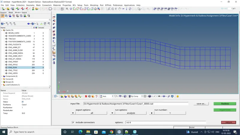
For Case 1 simulation, the given _0000.rad file was imported in the Hyperworks. Then as given in the question, the end time of the simulation was changed to 55 ms. To do this, under the model tree, 'cards' tab was opened and the "ENG_RUN" option was clicked. Then in the entity window, 'Tstop' was changed to 55 as shown below:

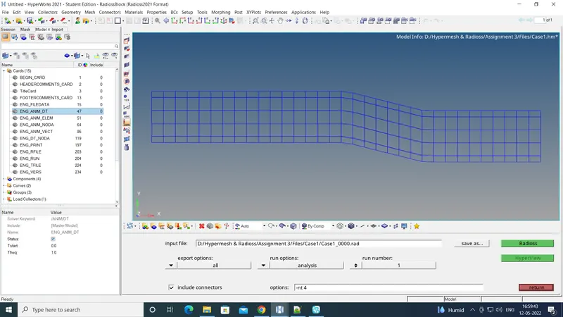
The the frequency of animation was to be kept in the range of 25-60 as per the question. To do this, under "Cards" in the model tree, "ENG_ANIM_DT" was opened and in the entity window, "Tfreq" was kept as 1.0. With the end time of 55 ms, this gave the frequency of animation as 55. This is shown below:

Then the model was run. To do this, on the Tools panel, "analysis" was clicked. Under this, "Radioss" option was selected. In this, 'include connectors' was ticked, export options was changed to 'all' and the 'options' tab, "-nt 4" was entered. The "Radioss" button was clicked. The simulation ran smoothly and terminated normally. Then in the Radioss console window, the energy error and mass error were checked.

Energy error = -10.3%

Mass error ratio = 1.659 e-4

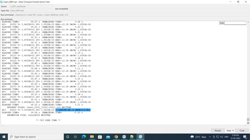
These values are in the acceptable range, close to 10% and the energy error is negative, indicating no addition of artificial energy. Also the mass error ratio is very very small, indicating very small addition of mass.

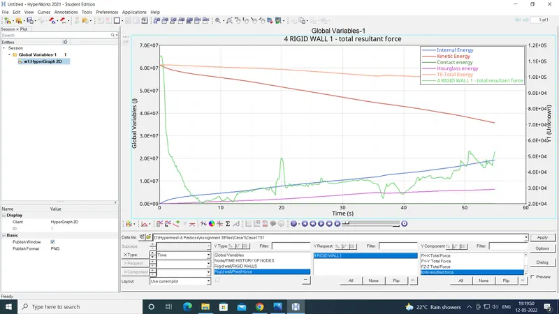
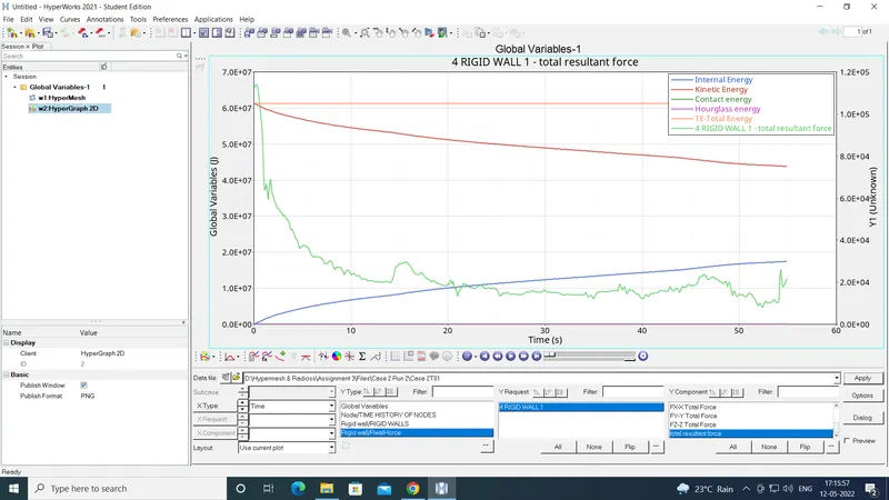
Then the graphic window was split in two parts and in second part, Hypergraph 2D was opened. In this the Case1T01 file of time history was opened. To plot energies, global variables were selected and internal, kinetic, total, contact and hourglass energies were selected. The MAG option was selected and apply button was clicked. This plotted the energy plots against time.

Then the Rigidwall force option was selected. Then total resultant force was selected and apply button was clicked. This plotted the rigidwall force vs time curve. The graphs are shown below:

Case 2:

This case involved inputting the recommended element properties. To do this, the given _0000.rad file was imported and the end time and animation frequency were changed as explained in Case 1.

To input the element properties, a DEF_SHELL card was created. To do this, from Menu bar, "tools" was selected. Under this "Create cards" was chosen, in which "control cards" was chosen, under which the "DEF_SHELL" card was chosen.

Then in the Model browser, under "Cards" "ShellDefault" was selected, and in the entity window, the recommended property parameters were input as shown below:

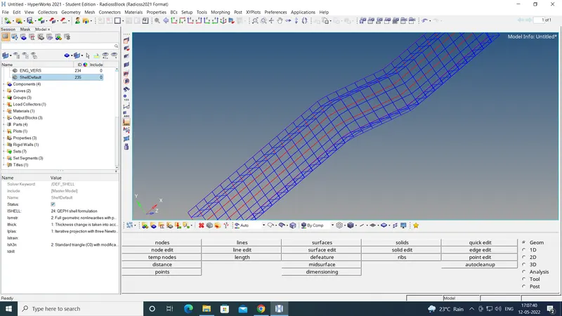
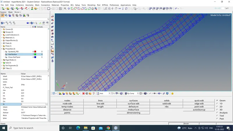
Then to select the value of N=5, under the ''Properties" tab, the 2 shell sections were selected individually and in the entity window of each, N=5 was input. This is shown below:

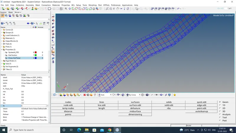
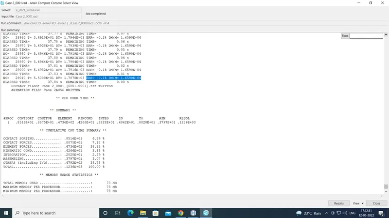
After this the model was run using the procedure as in Case 1 and the results were checked.

Energy error = -0.1%

Mass error ratio = 1.659 e-04

The plots for energies and rigid wall force are shown below:

Explanation of results:

The plots for both the cases are attached below:

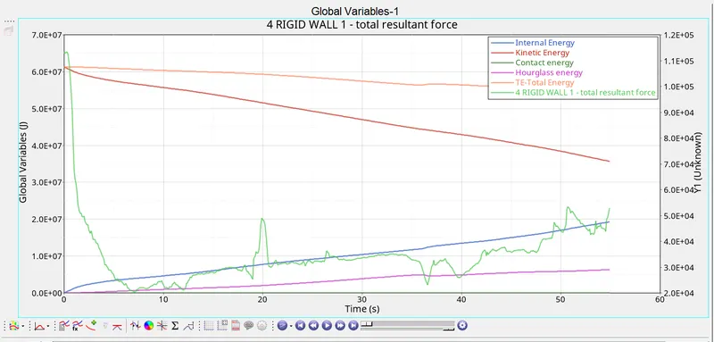
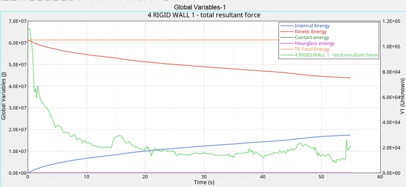
It can be seen from the above graphs that, although the initial values of energies and force are equal in both the cases, the final values are different.

The Case 1 uses the Q4 shell element which uses reduced integration and has only 1 integration point on the surface. This causes the accuracy of the simulation to be low.

Hourglass explanation: Also the Q4 element uses the perturbation method of hourglass control, which induces an artificial stiffness in the elements to counter hourglassing. This produces the hourglass energy in the system. Hence the energy error in the Case 1 is very high compared to the Case 2. Also due to increased stiffness of the elements, the rigidwall force also has higher magnitude than that in Case 2. Hence it also increases with the increase in hourglass energy.

On the contrary, in Case 2, QEPH elements are used, which use the stiffness method of hourglass control. In this method, the material properties themselves are adjusted to counter the hourglassing. This reduces the artificial stiffness and the hourglass energy added in the system. Hence in Case 2 the hourglass energy and the energy error are very low. Hence the total energy of the system remains almost constant, which is the ideal case, indicating the accuracy of the results.

Also the QEPH shell elements use the improved under-integration, which also increases the accuracy with maintaining efficiency. Hence the Case 2 results are more accurate. Also since the artificial stiffening is low in Case 2, the rigidwall force is also low in magnitude than in Case 1.

Hence it is clear that QEPH elements offer a good way to reduce the hourglass energy.

Conclusion:

Thus the results of the 2 simulations make it clear that QEPH shell elements are better in terms of accuracy and maintaining a reasonable efficiency. Thus the challenge clearly brings out the difference between the Q4 and QEPH elements. Also it was a good learning opportunity to familiarize with running a simulation using Hyperworks.