Assignment 3-2D Element Formulation Challenge

AIM: To run the simulation for the given component with and without changing the recommended element parameters using a raioss solver. 

OBJECTIVE:

• To change the run time to 55ms and to change the number of animation steps to 60.
• To run the basic simulation with default element parameters.
• To check the energy error and mass error for the base simulation.
• To plot the graphs for kinetic energy,internal energy,hourglass energy,total energy,contact energy and rigid wall forces.
• To run new simulation with recommended element parameters and to plot the graphs again.

THEORETICAL FRAME WORK:

Element formulation:

• Discretization is the process of dividing a model body into an equivalent system of many smaller bodies (finite element) interconnected at points (nodes or nodal points) common to two elements.Suppose we need to find the stresses and displacement upon loading an object with an arbitrary shape.So in order to model this,we need elements that have a geometric shape similar to the real structure or region.
• One geometric shape cannot represent all possible engineering structural shapes.The user will model with elements that look like a beam,truss,plane,cylinder etc.In FEA by using basic element almost all structures are approximated.The different element formulations (1D,2D,3D) require different parameters to be set.
• An understanding of FE elements,their types and their capablities is the first step to ensuring that the performance of the model is as close to the performannce of emprical study as the numerical will allow.The basic set of information output from a run includes stress and dtrain and physical displacement  and rotation.
• Ridios element library contains elements for one,two or thee dimentional problems and can be classified into the following categories of elements.

1. 3D Elements - Tetra,Penta,Pyramid,Hexa
2. 2D Elements - Trias,Quads
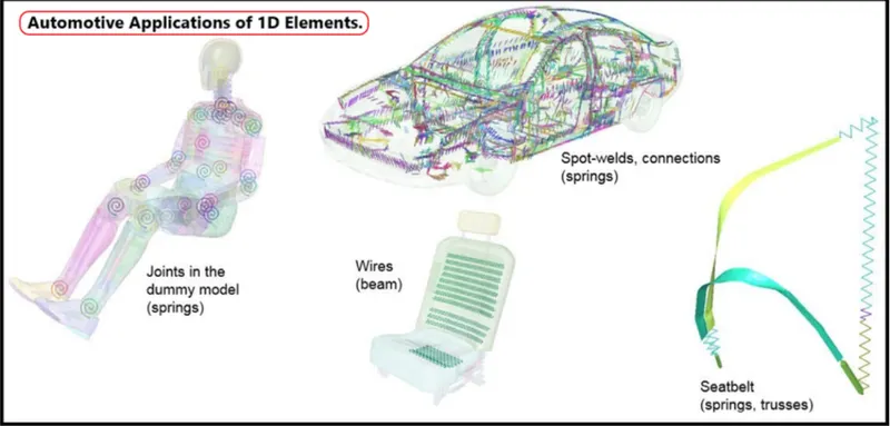
3. 1D Elements - Springs,Beams,Trusses

1D Elements:

• 1D elements are modeled by connecting two nodes together lineraly and then assigning constant cross-sectional properties to that element to define the element's behaviour.
• There are three types of 1D elements available- Truss elements, beam elements and spring elemets.

Truss Elements:

• Truss is a 2 noded elements.
• Tensile/compression behavior only (no bending stiffness)
• Compatible with elastic and elastoplastic materials (law 1 and 2)
• Property define by cross-sectional area
• Force output in truss orientation
• Truss is used for modeling cables,ropes,chains

Beam elements:

• It's property is defined by cross sectional area and inertias.
• The 1,2 node defines element geometry,the 3 node defines the cross sectional orientation.
• 6 DOF's per node (bending and torsional stiffness)
• `omega`DOF: flags for release of rotational stiffness at end nodes.
• Based on the timoshenko formulation,can degenerate into the standard Euler-Bernoulli formation.
• The existence of bending stiffness is the primary difference between beam and truss elements.

Spring Elements:

• Spring elements are also 1D elements that are modeled using 2 nodes.These elements are commonly used to model connectors in the model.
• Simple physical spring with a dashpot
• DOF per node undergoes tension and compression behavior.
• Linear elastic.
• Nonlinear elastoplastic.

2D Elements:

• Shell elements are 3 or 4 node 2D planar elements with constant thickness and have either a triangualr or quadrilateral shape that can be oriented in the space.
• They are typically used to model structures such as press vessels,automobile bodies,ship hulls,aircraft fuselage etc.
• Shell elements supports all translational degrees of freedom as well as all rotational degrees of freedom that is shell elements have 6 degrees of freedom,Ridioss shell are based  on mindlin-reissner theory that includes transverse shear eformation valid for moderately thick and thin shells.
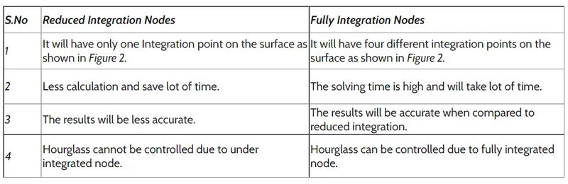
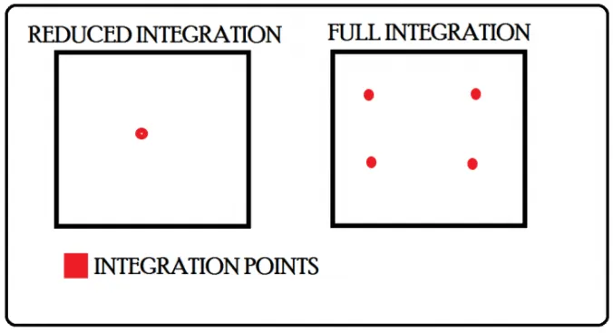
• RADIOSS provides both reduced and fully integrated 4- noded shell elements.

Reduced and Fully Integration Nodes:

Hourglass:

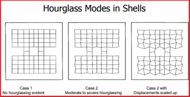
• Hourglass deformation happens to a element due to a applied load.
• It is excessive deformation in finite element mesh.
• Element having zig-zag or hourglass like shapes.
• Hourglass deformation occurs due to an under integrated nodes. Explained above what is under integrated node,reduced integrated node and fully integrated node.
• Under integrated node is nothing but reduced integrated node.
• Hourglass can occur in 2D or 3D element (reduced integration scheme) when subjected to bending load.

• 

Methods to control Hourglass

There are two methods to control hourglass deformation called

1) Pertubation method Ishell=1,2,3 or 4(Q4) [Viscous method]

• The hourglass deformation is detected with the relative motion (velocity) of the nodes.
• When hour glassing is detected,a force is applied on the node to stablize the deformation.
• This force is defined according the element stiffness (young modulus,yield stress, plastic tangent)
• This force ntroduces an artificial energy (named hourglass energy)

2) Pertubation method Ishell=24(QEPH) [STIFFNESS METHOD]

• Hourglass yiel depends on natural yield.
• Hourglass loading stiffness depends on natural tangent modulus.
• The hourglass treatment is done at the material level.
• QEPH is not recommended for orthotropic materials.

[Note: hourglass should not exceed 5% of internal energy]

2D Element formulations:

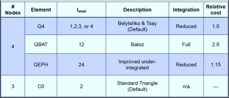
Key parameters for shell elements:

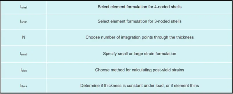
Q4 Element:

• Integration points on the surface.
• Relatively inexpensive.
• Default shell formulation is Ishell = 1.
• Q4 is an under-integrated 4 node element (BT)
• Hourglass stablization with pertubation method.

QBAT Element:

• QBAT is a fully integrated 4 node element (Batoz).
• 4 Gauss integration points on the surface.
• No hourglass deformation.
• 5 local degrees-of-freedom per node- drilling( rotation around ocal z) can be activated with Idrill.
• No shear locking due to in plane reduced integration for shear.
• Transverse shear deformation is taken into account.
• Most accurate element,but higher CPU cost (2 to 3 times that of a Q4).

QEPH Element:

• QEPH is an improved under-integrated 4 node element with 1 integration point on the surface.
• Physical hourglass stablization.
• Best compromise between cost and quality.
• Generally,QEPH elements costs only up to 15% more than a BT element and the results are close to those of QBAT.

CO Element:

• CO is a standard triangle (CO) with modification for large rotation.
• 1 integration point on the surface.
• No hourglass deformation.
• Low CPU Cost.

N- No. of integration points through the thickness:

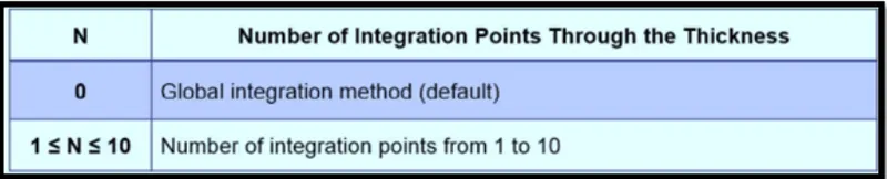
• Up to 10 points through the thickness.
• 1 integration point through the thickness give membrane behavior.
• N= 5 integration points recommended.

Shell strain formulation Ismstr:

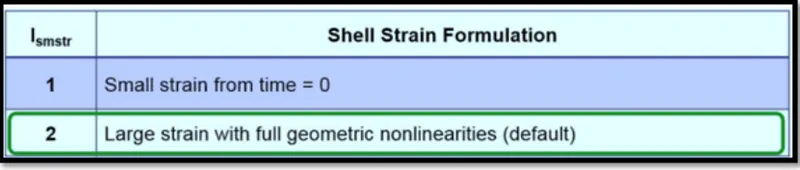
Small Strain-

• Usually for problems with small deformation.
• Strain computed based on the initial element shape.

Large strain-

• For problems with large deformation and starin.
• Strain computed based on the current element shape with the derivate of the shape function.
• Small strain activation possible in Radioss engine in the event that time step reaches D Tmin due to element deformation.

Shell Stress Computation -

• From the deformation and the strain rate of the previous tep, Radioss computes the strain to each integration point.
• From this strain,the stress is computed with a elastic stress increment.

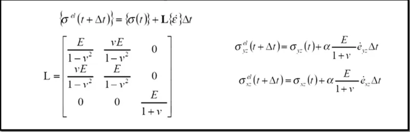
• With these computed stress values,the Von mises stress is computed and compared to the yield stress of the material. 
• If the von mises stress is similar than yield stress,the computed stress is the one used in order to compute the internak force of the elements.

Shell plane stress Plasticity Iplas-

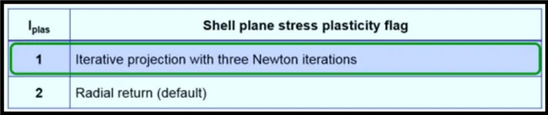
• If the Von mises stress is bigger than yield stress,RADIOSS will:

• Update the strain through the thickness.
• Compute the new thickness of the shell element.

• Compute the stresses using the material law plasticity surface,the strain and the strain rate.The projection of the stress on the plastic surface is done with:

• Radial return (faster)
• Iterative.
• Projection with Newton's method.
• More accurate.

Thickness change Ithick -

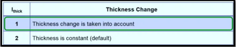
Intitial thickness is used to compute starins and to integrate stresses but the thickness variation is still computed for post-processing reasons.

If a variable thickness is used,true thickness is computed not only for postprocessing but also for strain computation and stresses integration.

For accurate results,especially when necking or spring back,it is stronglyrecommended to use iterative plastic projection and thickness variation.

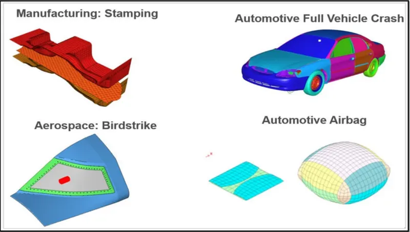
Shell Elements Recommendations for Crash Application -

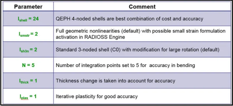
Shell Elements Recommendations for Crash Applications:

PROCEDURE:

Phase 1- Import the starter file into the solver deck radioss

• While operating hypermesh software. A user profile window will pop up. Switch to the radioss user profile as shown in below figure and start importing the model into the solver deck.

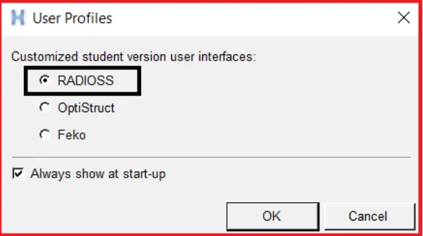
• Now after switch the user profile to radioss.import the model (starter file) into the radioss solver deck.
• To import the model, go to standard panel>>Import>>Import solver Deck.

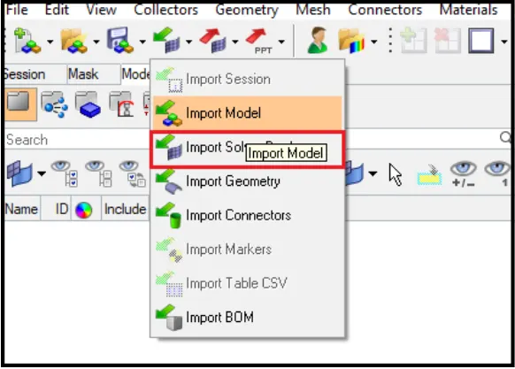
• Import solver deck option should be selected to import the radioss starter file

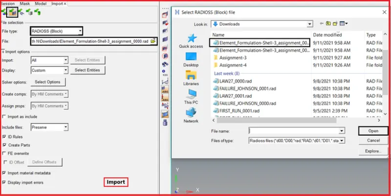
• Here the import browser will appear as shown above figure. select the appropriate starter file to import into GUI.
• Switch the file type to RADIOSS block and import the model into GUI.

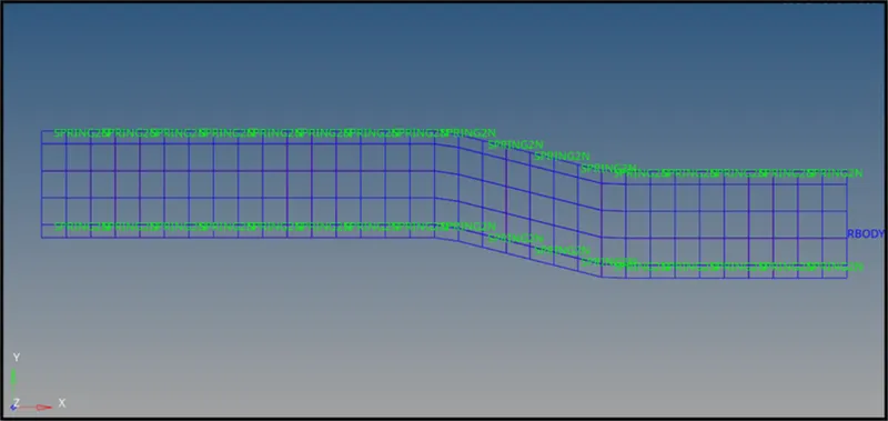
• Here the model is in wireframe mode,switch to the shaded mode as shown in below.
• To switch the shaded mode,go to visualization tab>shaded elements and mesh lines.

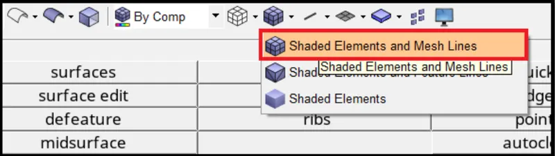
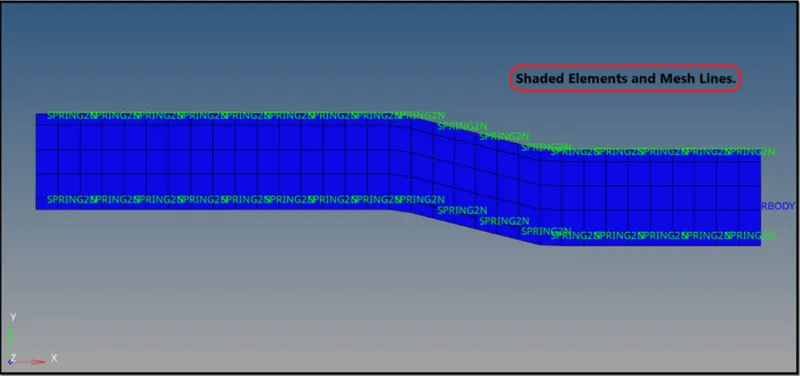
shaded element and mesh lines mode

Phase 2- Edit ENG_RUN File [Tstop] and ANIM_DT [Tfrequency]:

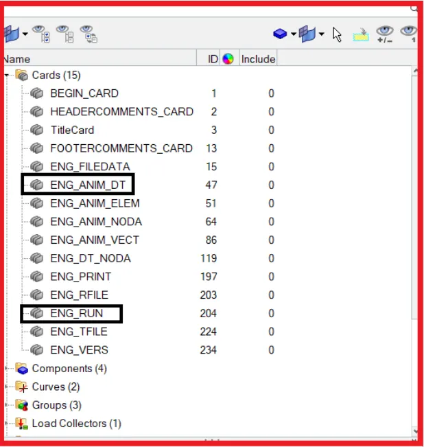
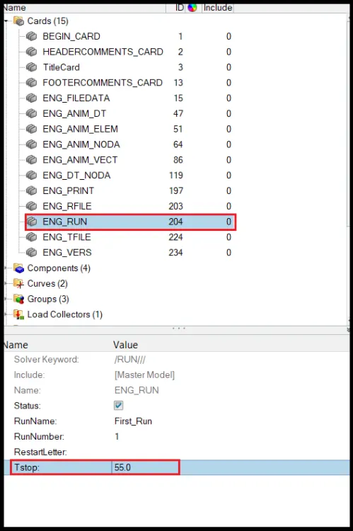
• As per our requirement,we need to change the Tstop value and Tfrequency value.
• To change the values,go to model browser>control cards>edit the values by selecting the appropriate control card.

1) Run time [Tstop]

• Run time is the total time taken for the sound wave to travel through the entire length of the model.
• Time for sound to travel length of rail formula is deltat=L/C

Where delta t= time step

L= length of the rail

C= speed of the sound

Here the Tstop=55ms value has been already given in the question,so need to calculate.

Enter the value 55 in ENG_RUN File which is shown in the below fig.

2) ANIM_DT[Tfrequency]:

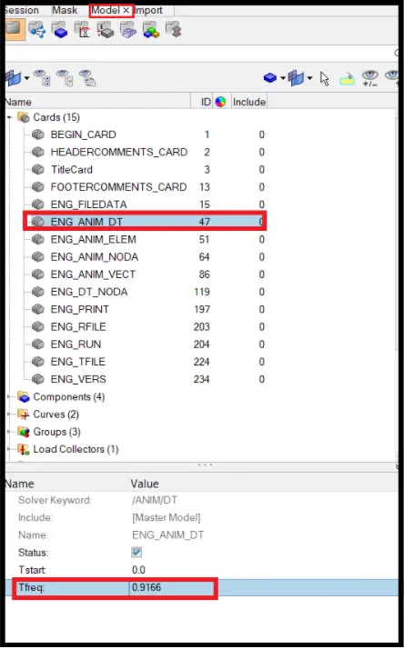
As per our requirement,engine file have to generate between 25-60 animation files.

Here we are taking value 60,the solver will create 60 animation files within the termination time.

Tfrequency= Runtime/ Number of animation steps

Tfrequency= 55/60

Tfrequency= 0.9166

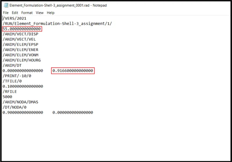
Now go the model browser>select appropriate control card >ANIM_DT> enter value as 0.9166 as shown in the figure.

Phase 3- Run the base simulation with and without changing the recommended shell parameters

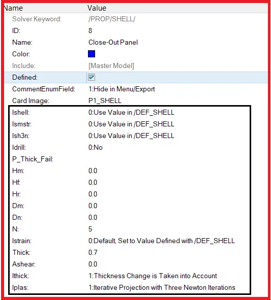
case 1- without changing the recommended shell parameters.

• Run the base simulation with default shell parameters as shown below,don't assign recommended shell parameters.

• Now run the simulation,to run simulation,go to analysis panel as shown in fig.
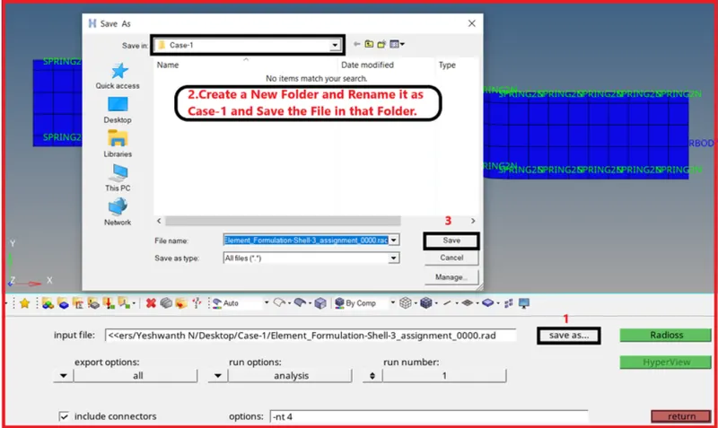
• Go to analysis panel>radioss>select the input file>save it in different folder and rename it as case1>run.
• Check the include connectors,if there are any connectors in the model.The connectors will also be taken ino account.
• Type -nt 4 in options tab,this will make the simulation faster.
• Where nt indicates no of threads,4 indicates assigning the task to 4 cores in the system.

• Here save the input file in a different folder,and rename it as case-1 which is shown in below.
• Now run the solver by hitting on radioss.

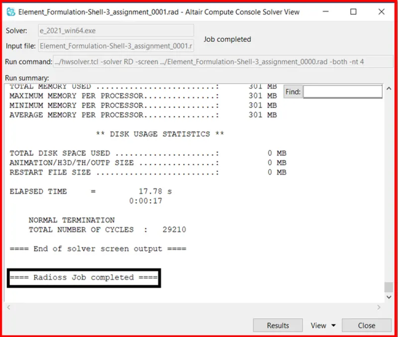
• After completing the simulation,the radioss will pop up a solver window stating Radioss job completed which indicates the simulation has been completed which is shown below fig.

• Now verify the Tstop and Tfrequency values are properly assigned in engine.rad file [00001.rad]
• Open engine .rad file [00001.rad] with notepad as shown in below fig.

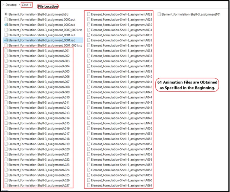
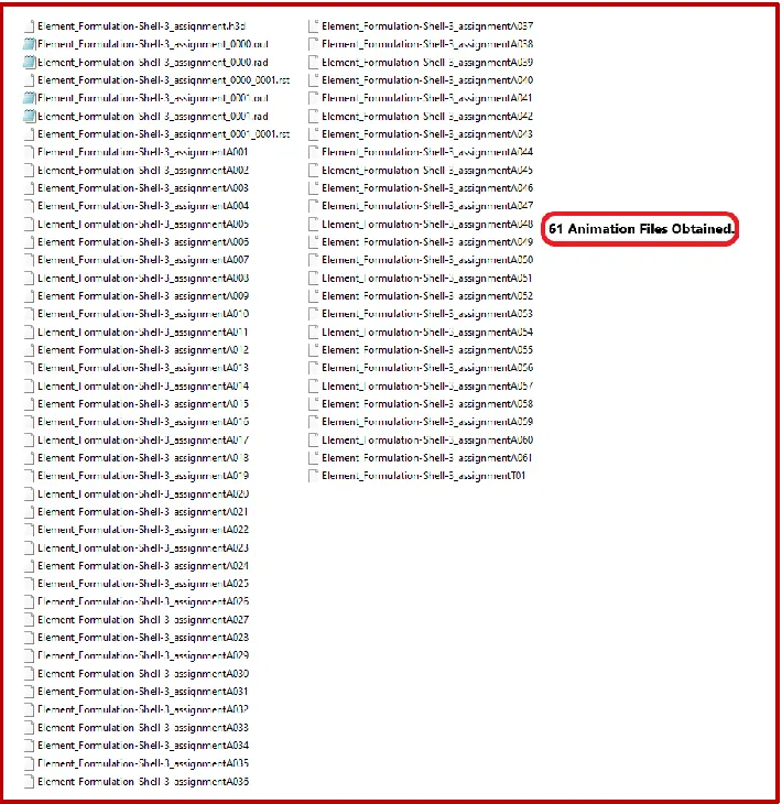
• Next verify the required number of animation steps obtained in the file location or not.
• In the begining the specified number of anmation steos was assigned as 60.
• Here the number of animation steps obtained are 61 which is shown in below fig.

Phase 4- Do energy error and mass energy error checks

• Now engine output file [00001.out] has been generated after analysis.
• The engine output file [00001.out] contains the data like

1. Time step
2. Energy Error
3. Mass Error
4. Internal energy error
5. Kinetic energy error
6. contact energy error

• Here check the mass error and energy error.
• The obtained values for energy error,mass error,internal energy error,kinetic energy error and contact energy error has been shown in below fig.
• The acceptable energy error range is -15% to +5%.
• The acceptable mass error rnage is 0 to 2%.

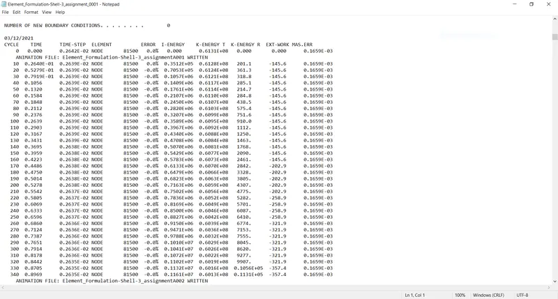
Scroll down to see the maximum value obtained for the energy error,kinetic energy error,internal energy error and mass error as shown in below figure.

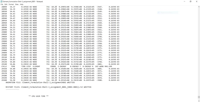
• The maximum energy error is = -10.3%
• The maximum internal energy error = 0.1932 x 
• The maximum kinetic error = 0.3563 x 
• The maximum mass error = 0.1653 x 

Note:

1. The acceptable energy error range is -15% to +5%.
2. The acceptable mass error rnage is 0 to 2%.

Now these two error values are acceptable,they are not going beyond the standard values.

Phase 5- Postprocessing

1) Review the simulation using- Hyperview.

2) Plot the graphs using- Hypergraph 2D

Review the simulation using Hyperview:

• Hyperview allows for loading and viewing result obtained from several sources.
• Based on the solver type of the files and the results you would like to visualize and analyze,there are different ways to load the input deck and their corresponding result into hyperview.
• First to begin in the postprocessing in the hypermesh split the screen as shown below.
• Import the animation file.h3d into hyperview.

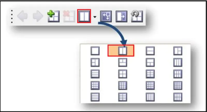
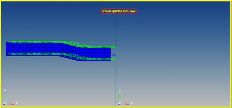
• And then activate the client Hyperview

• To access the load model panel.
• Select load model button from the hyperview panel and open .h3d file as shown in below fig

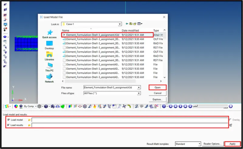
Opening .h3d File.

After loading the model into hyperview,it will be represented as shown in fig.

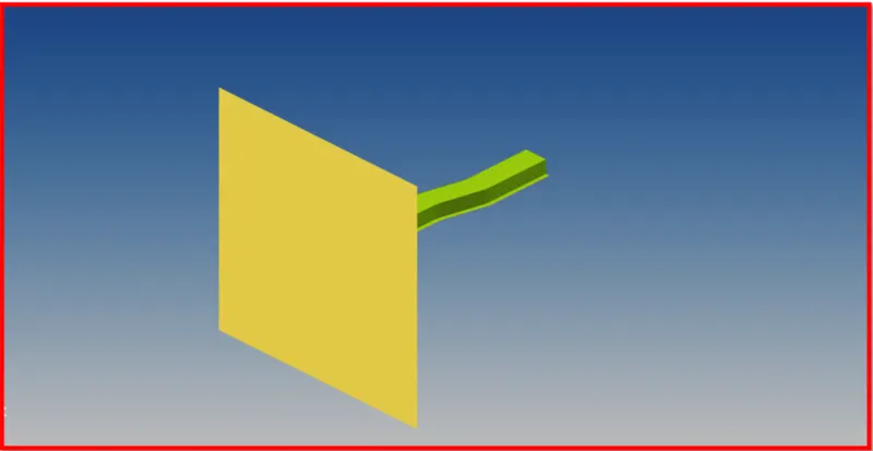
• After importing the .h3d file into the GUI. enable the contour.
• The contour tool create contour plots of a model graphically visualize the analysis results.
• To enable contour. Go to results toolbar> contour.

• Now switch to the von misses -stress in result type and select the component,select the averaging method as simple and then click apply as shown in below.

• After applying,Run the simulation,the simulation animation is shown in below.

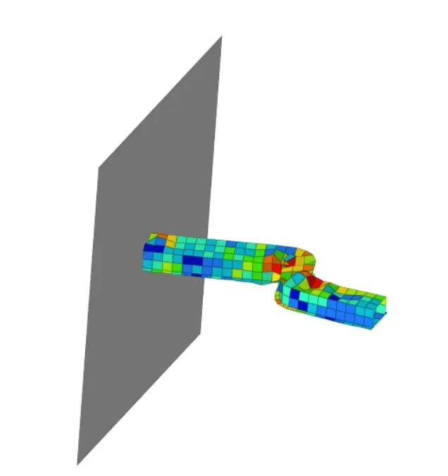
2) Plot the grapth using- Hypergraph 2D

• Now plot the graph using hypergraph 2D,we are plotting the graphs to see what is happening in the rail component.
• Hypergraph 2D is a powerful data analysis and plotting tool with interfaces to many popular file formats.
• It is sophisicated math engine capable of processing even the most complex mathematical expressions.
• Hypergraph 2D combines these features with hogh quality presentation output and customization capablities to create a complete data analysis system for any organization.

• Here switch to the hypergraph 2D to plot the graphs.
• To switch,go to client selector>>choose the hypergraph 2D as shown above.

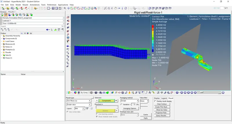
• The first graph is plotted for the rigid wall forces.
• To plot the graph,go to hypermesh 2D>> data file>> element_formulation-shell-3_assignmentT01>> Apply.

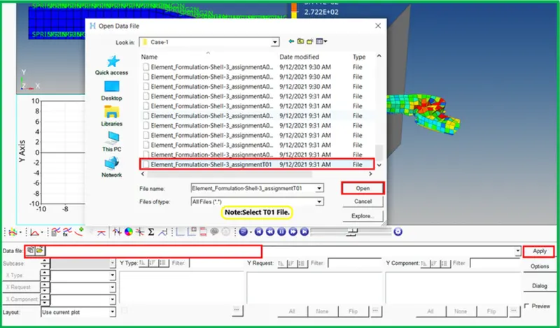
• Here the graph has been plotted for the rigid wall forces as shown in below fig.
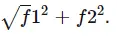
• There are various parameters in rigid wall like normal force.Tangent force.FX-X Total force,FY-Y total force,FZ-Z Total force,total resultant force.
• We are selecting only total resultant force because we dont know the exact axis of the component placed,so that's why we are selecting total resultant force and then plotting the graph.

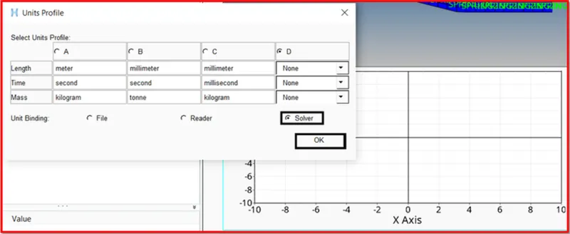
• While plotting the graph,units profile window will pop up,there select solver units and then plot the graph because the graph will be plotted according to the solver units.

Case 1- Without assigning the recommended parameters in the property.

Rigid Wall Forces:

• Total resultant force= 
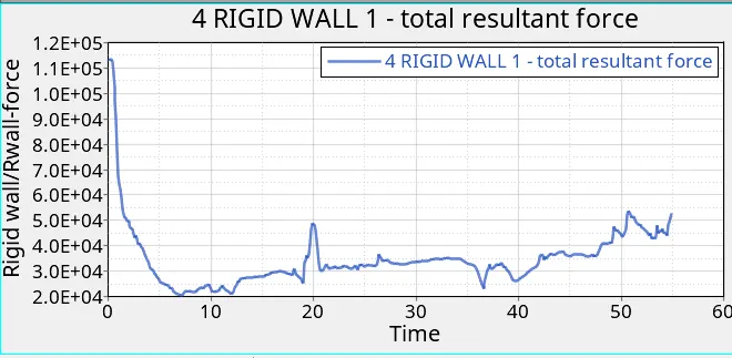
• Rigid wall forces are the forces which are acting on the rigid wall.
• Here the rigid wall forces is at higher value in the begining.
• In begining there is no impact in the simulation,but in the graph the rigid wall forces are at the higher values.
• This is because,the solver didn't record in that time,so the rigid wall force is at higher value in the begining.
• When the rail component hits the rigid wall,the rigid wall forces increases from the begining.
• It goes on decreasing,because the deformation is happening to the rail component when it hits to the rigid wall.

[Note: The solver starts to record when the rail component hits on the rigid wall,this is the reason why in the begining,the rigid wall forces is higher value or increases and goes on decreasing.]

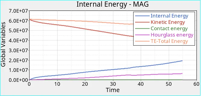
Next plot the graphs for the kinetic energy,internal energy,total energy,contact energy and hourglass energy.Those graphs are plotted and shown in the below fig.

 

Kinetic Energy:

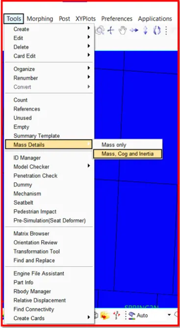
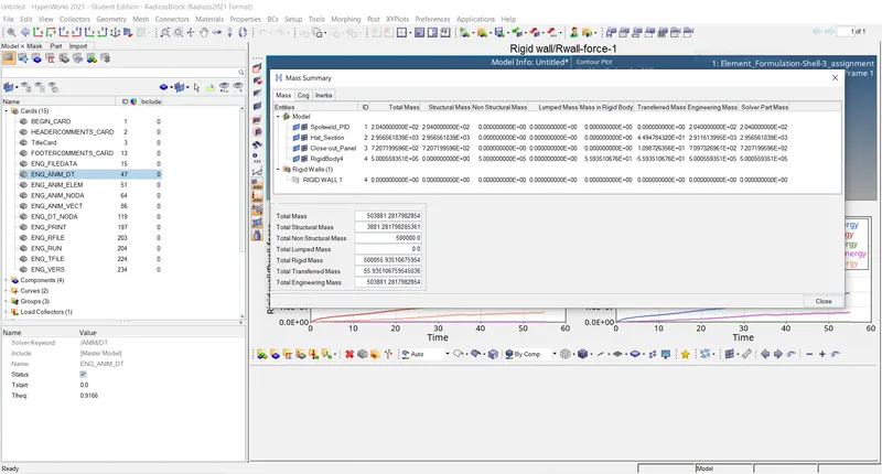
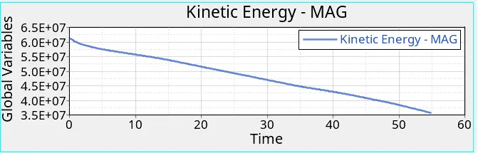
Kinetic energy is at peak in the starting,why because we have huge mass which  is shown in below.

To check mass,go to tool>>mass details>>mass,mass,COG,Inertia.

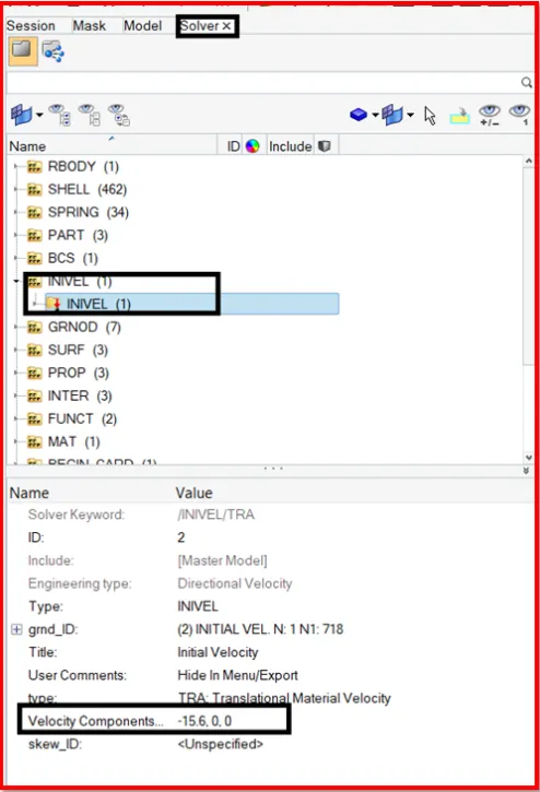
To check velocity,go to solver brower>>INIVEL Card>>Initial velocity.

• Kinetic energy is lower and decreases,why because there is a velocity applied to the component,so its getting deformed and the kinetic energy decreases.
• The formula for kinetic energy= 1/2 MV*2
• Given data
• Mass= 503881.28179g
• Velocity= -15.6ms
• KE= 1/2 X (503881.28179)(-15.6)*2
• KE = 61312274.37
• The value calculated here is shown in the fig.
• With the calculation,we came to know why kinetic energy is increasing in the begining itself,why because the initial velocity is given for the component.
• The kinetic energy decreases,why because the velocity decreases( the rail component starts to deform,after complete deformation,it will be in rest) when the component comes to a rest,so velocity becomes zero and the kinetic energy decreaes.

Internal Energy:

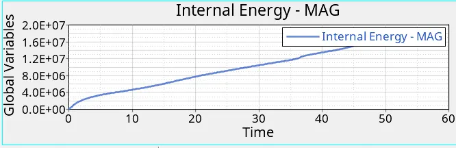
• The formula for internal energy is E=Q+W
• Here the heat is neglected,cause there is no heat transfer,we will be having only workdone.
• W=FXD
• Here the internal energy is in zero,because there is no deformation initially,so the internal energy is in zero and starts from zero and goes on increasing.
• The internal energy increases because the dformation is happening there is a displacement,so the internal energy increases,when the displacement or deformation occurs.

Total Energy:

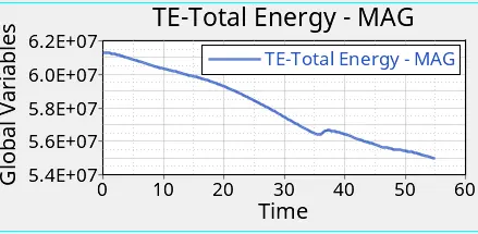
• Here total energy starts from the higher value,in starting itself its increasing why because the total energy is sum of kinetic energy+contact energy+hourglass+internal energy.
• All energies are in initial condition except kinetic energy,so kinetic energy is only there.
• Total energy= kinetic energy+0+0+0.
• Kinetic energy is directly proportional to the total energy.
• SO the toatal energy is increasing in the begining.
• Due to 10.3% of energy error,the total energy is decreasing.

 

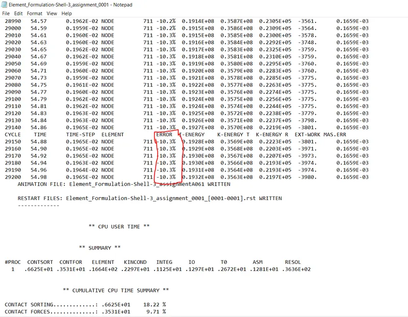
• Why it is decreasing.let's see mathematically
• energy error=10.3%
• 10.3/100 x61314900.
• =0.103 x 61314900
• = 6315434.7
• Now subtract this value with maximum total energy error.
• Total energy error maximum value = 61314900
• =61314900-631543.7
• =54999465.3
• We got an minimum value which is shown in above fig.

 Contact Energy:

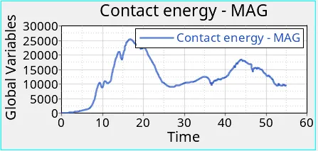
• Here the contact energy starts from origin,cause the rail component is in intial condition.
• Intially there is no contact between the rail component and rigid wall.
• There is also no deformation intially but when the component goes and hits on the rigid wall,the contact energy starts increasing.
• When the deformation or dispalcement happens to the component,the contact energy increases cause the crash tube or rail component comes within the contact to the rigid wall,so the contact energy goes on increasing.

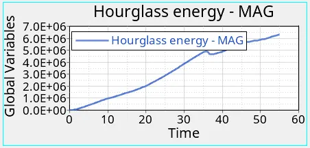
Hourglass Energy:

• delta t> t - hourglass exsist.
• delta
• Where deltat- shockwave
• t- time taken for the information.
• Here the hourglass energy is starting from origin because the recommended parameters has not been specified.
• The hourglass energy goes on increasing because to balance the rest of energies.An artificial energy is required that is called hourglass energy and thats's the reason why hourglass energy goes on increasing from origin.
• A lot of hourglass energy is needed,so its goes on increasing.

 Case 2- With assigning the recommended parameters in the property.

• Now enter the recommended parameters in properties called Hat-section,close-out section which is given in the question.
• The recommended parameters have been entered in the properties as shown below fig.

   

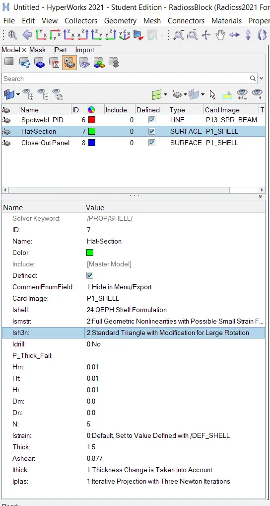
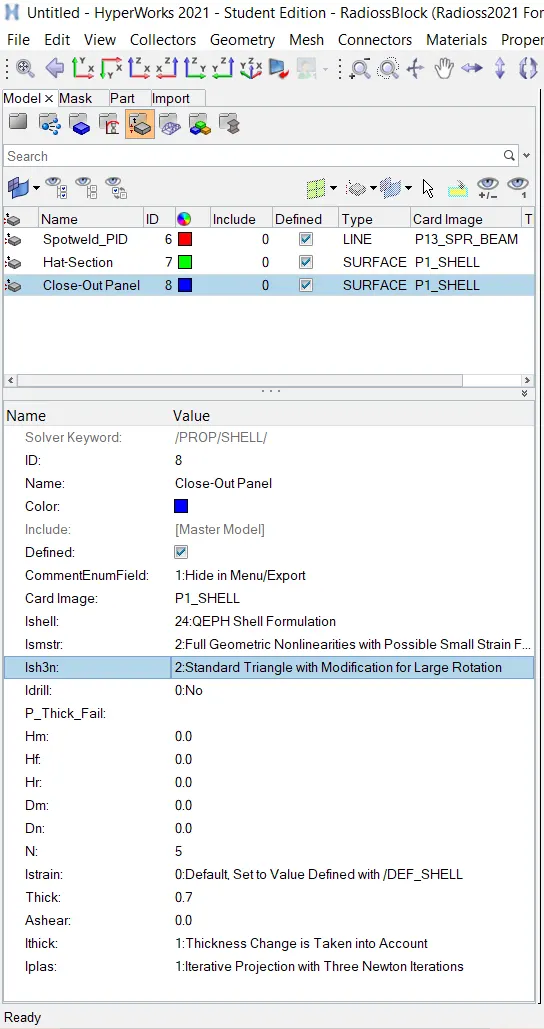
• Similrly follow the same process and do the same what we have done for the case 1.
• Now run the simulation for the case 2.

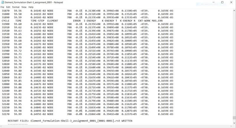
• Now go open the engine output file to check whether there is improvement or not.
• There is improvement when compared to the values obtained from case 1.
• Here the energy and mass error values are acceptable and start to run the simulation.

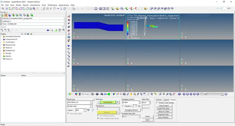
• Now run the simulation,to run simulation we need a additional window.In the main page menu,go and split the window into 8  as shown in fig.
• In any new window switch to hyprview and then load the .h3d file.The loaded .h3d file is shown in fig.

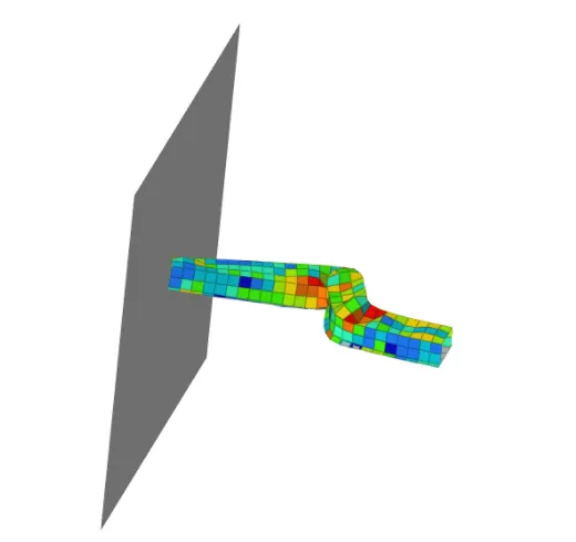
• Now run the simulation and in the result type switch to the von misses stress as shown in below fig.

• Now plot the graphs for the energies, to see the changes in the results with respect to the case 1 plot the graphs for all the energies.
• Here the graph has been plotted for the rigid wall forces which is shown in below fig.
• Similarly plot the graphs for all the energies.

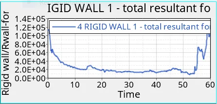
• Here there is little bit improvement after assigning the recommended shell parameters when compared to case 1.
• Here, there is no hourglass effect due to recommended parameters,so the rigid wall forces curve is again increasing,if you compare the case 1 and case 2 simulation animation properly,you will get an idea.
• The graph has been plotted for all the energies like kinetic energy,internal energy,contact energy,total energy anf hourglass energy which is shown in below fig.

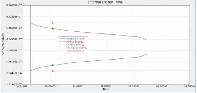
• Here there is a little bit of improvement in all the enrgies when comapred to the case-1
• Now plot the graph for the hourglass energy to see the result,whether there is any improvement in hourglass energy or not.

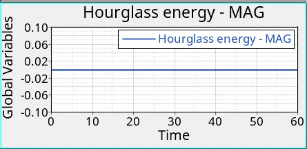
• Here the hourglass energy is constant,why because the recommended parameter Ishell= 24[QEPH 4 noded shell]
• It will be having 4 nodes in the element,so hourglass won't happen,it will be constant.
• In previous case,it was under integrated node,so there was hourglass deformation.

Final Image- 

Here in the case 2 graphs which is shown below,there is no much change.

   

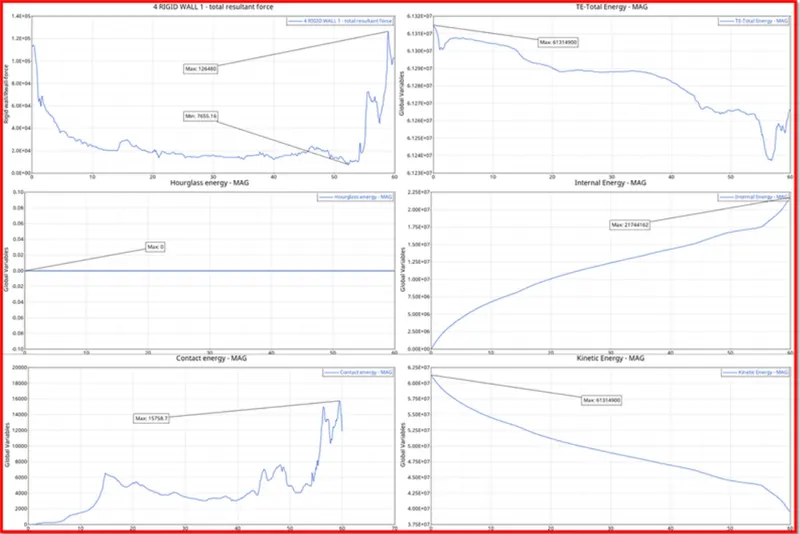
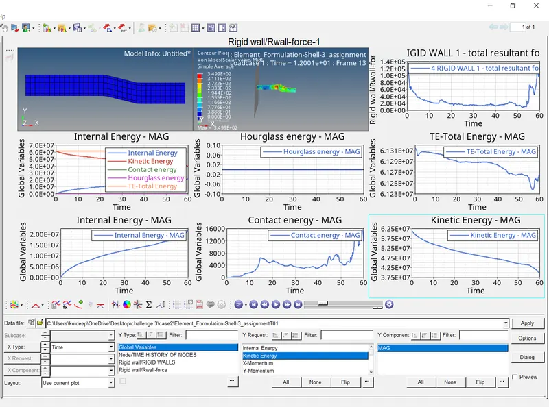
Comparison of case 1 and case 2 simulation.

S.No.	Characteristic	case-1	case-2
1.	Maximum energy error	-10.3%	-0.1%
2.	Maximum kinetic energy	0.3563E+08	0.3941E+08
3.	Maximum internal energy	0.1932E+08	0.2186E+08
4.	Total energy	Toatal energy increases and slighly decreases due to energy error	Total energy remains constant
5.	Hourglass energy	Hourglass energy increases due to balance all the energies	Hourglass energy remain constant due to recommended shell parameters.

Result:

• Hence the simulation has been runned without assigning recommended shell parameters.
• Hence the simulation has been runned with assigned recommended shell parameters.
• The graphs have been plotted for case-1 and case-2 successfully.
• While comparing case-1 and case-2,case-2 is effective,cause there is no hourglass deformation.

Conclusion and learning outcome:

• I conclude that case case-2 with assigning recommended shell parameters is effective.
• In this challenge,i came to know.
• How to run a simulation with and without assigning shell parameters.
• How to do postprocessing (plotting the graphs for the various parameters).
• How to understand the curves that are increasing and decreasing in the graphs.
• How to compare the obtained values with the various parameters.