Comparison of simulation results
AIM:
To compare the simulation results of CASE 1 and CASE 2 i.e, without changing element properties (CASE 1) with improved shell element properties
(CASE 2).
SOFTWARE:
HyperWorks 2020
USER PROFILE:
RADIOSS
PROCEDURE:
CASE 1:
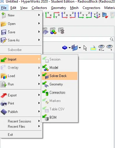
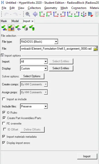
First import the starter file to HyperWorks. To import the file Go to "menu bar > File > import > solver deck, select the starter file, and click on import.
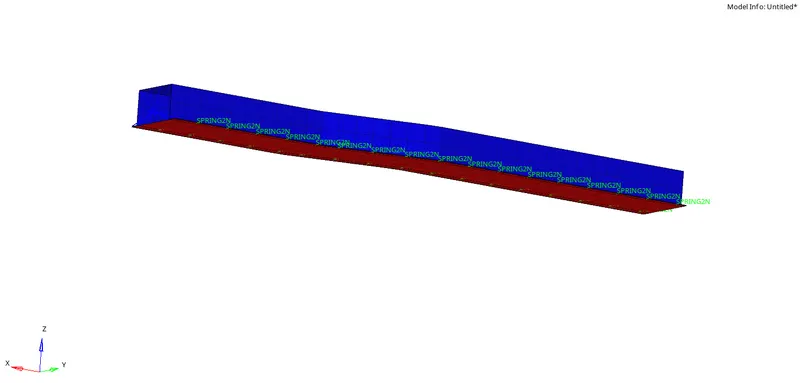
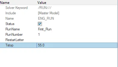
After importing the model, change the simulation stop time. To perform this operation Go to tab bar > cards > ENG_RUN > Tstop. Change the Tstop value to 55. This will change the run time.
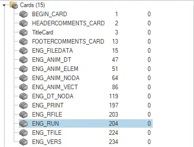
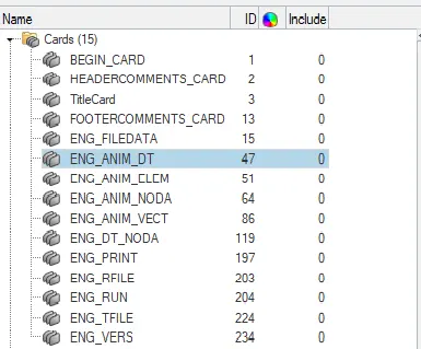
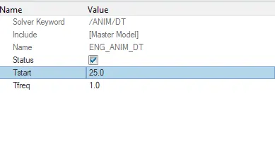
Now change the simulation start time to 25ms. To perform this operation Go to tab bar > cards > ENG_ANM_DT > Tstart. Change the Tstart value to 55. This will change the number of animation steps during simulation to a minimum of 25 and maximum of 60.
Now run the base simulation without any modification to element properties. To perform this operation Go to "main menu page > Analysis > Radioss.
Change the input file directory to a new folder (case 1). Tick the box of include connectors and under the options tab, type the values as -nt 4 and click on Radioss to run the simulation.


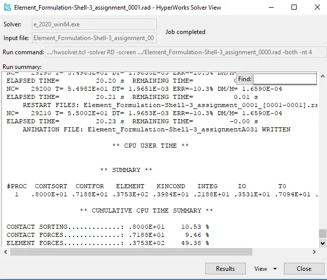
Once the simulation is run, HyperWorks will popup a box in which it will show the simulation process as shown in the figure below.
Now in order to check the animation, run the animation file in Hyperview(.h3d). Select this file from the directory folder (the new folder which we created for the input file directory).

Upload the .h3d file and click on 'Apply'.

Click on the play button to see the animation.
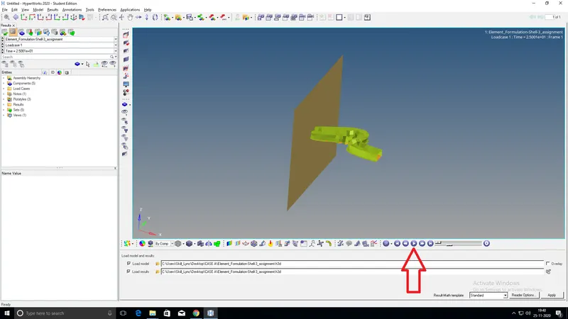
In order to plot rigid wall forces, internal energy, hourglass energy, contact energy, total energy of the simulations, open HyperGraph 2D.

Now update the TO1 file in HypherGraph 2D.
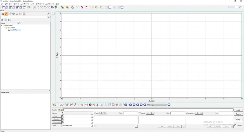
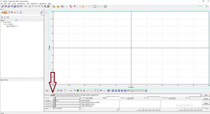
To apply rigid force refer to the below image.

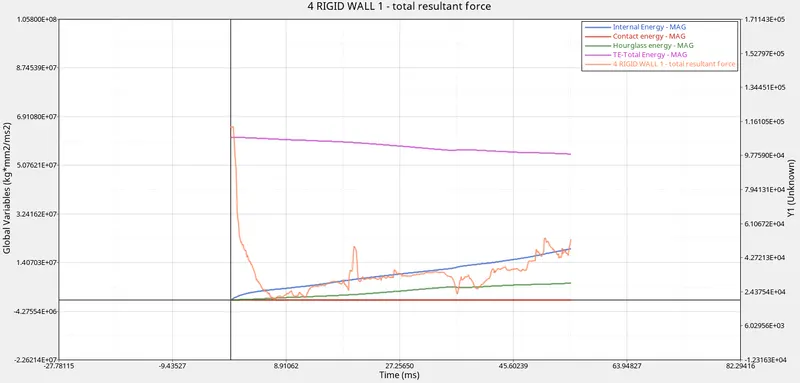
Similarly, all the other energies i.e, internal energy, hourglass energy, contact energy, and total energy can be applied from the global variables as shown below.

We need to select the units for these energies to plotting on a graph. The below figure which is showing the units table will appear on the screen once we apply energy.
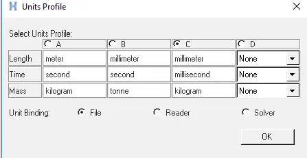
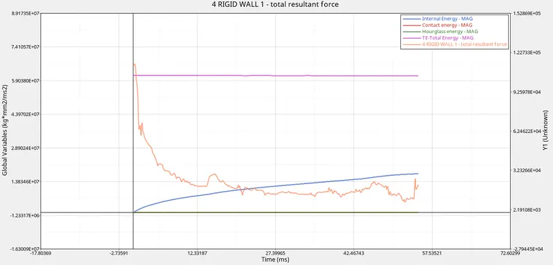
Below figure is the final graph for case 1 after applying all the energies.
CASE 2:
Similar to case 1 first import the starter file to HyperWorks. To import the file Go to "menu bar > File > import > solver deck, select the starter file, and click on import.
After importing the model, change the simulation stop time. To perform this operation Go to tab bar > cards > ENG_RUN > Tstop. Change the Tstop value to 55. This will change the run time.
Now change the simulation start time to 25ms. To perform this operation Go to tab bar > cards > ENG_ANM_DT > Tstart. Change the Tstart value to 55. This will change the number of animation steps during simulation to a minimum of 25 and maximum of 60.
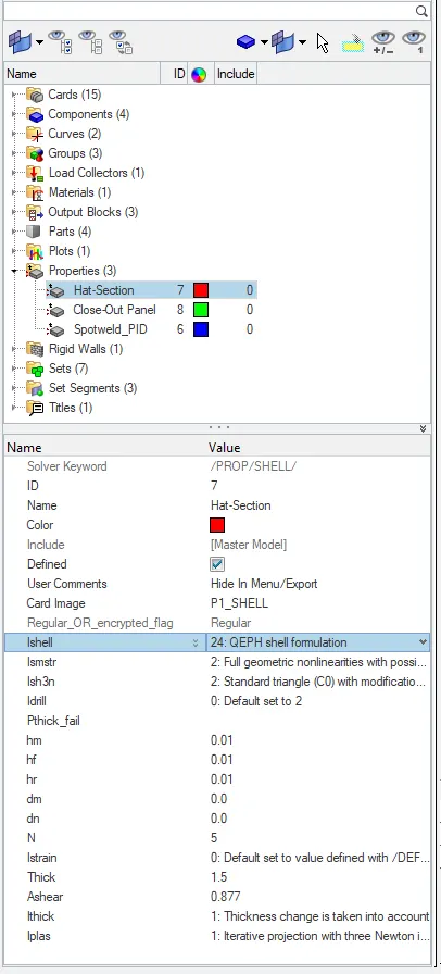
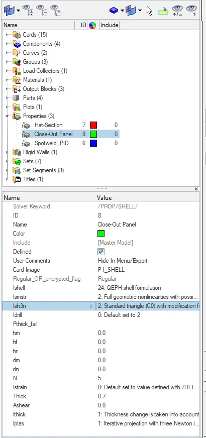
Now in this case before running the simulation, change all the shell elements properties to recommended properties. The given shell element properties are:
Ishell =24 - QEPH 4 nodes shells are the best combination of cost and accuracy.
Ismstr=2 - Full geometric nonlinearities (default)with possible small strain formulation activation in RADIOSS Engine.
Ish3n=2 - Standard 3 noded shell (C0)with modification for large rotation(default)
N=5 - Number of integration points set to 5 for accuracy bending.
Ithick=1 - Thickness change is taken into account for accuracy.
Iplas=1 - Iterative plasticity for good accuracy.
Now run the simulation with these updated properties. Change the input file directory to a new folder (case 2). Tick the box of include connectors and under the options tab, type the values as -nt 4 and click on Radioss to run the simulation.
Now in order to check the animation, run the animation file in Hyperview(.h3d). Select this file from the directory folder (the new folder which we created for the input file directory).

Now in order to check the animation, run the animation file in Hyperview(.h3d). Select this file from the directory folder (the new folder which we created for the input file directory).

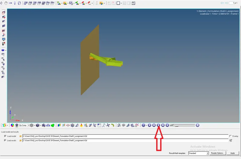
Click on the play button to see the animation.
In order to plot rigid wall forces, internal energy, hourglass energy, contact energy, total energy of the simulations, open HyperGraph 2D.

Now update the TO1 file in HypherGraph 2D.
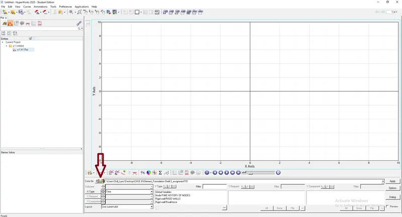
To apply rigid force refer to the below image.

Similarly, all the other energies i.e, internal energy, hourglass energy, contact energy and total energy can be applied from the global variables as shown below.

We need to select the units for these energies to plotting on a graph. The below figure which is showing the units table will appear on the screen once we apply energy.
Below figure is the final graph for case 2 after applying all the energies.
Comparison of case 1 and case 2:
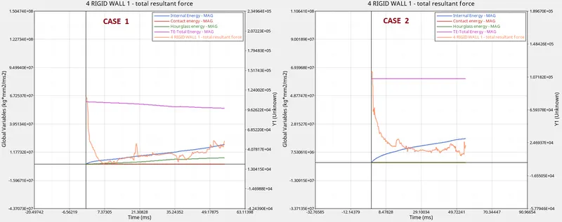
QEPH gives more accurate results in case of loading and unloading even if there is hourglass mode deformation. QEPH also has physical hourglass stabilization due to these reasons the hourglass energy is constant in case 2 and not in case 1.
Similarly due to the changes in element properties such as ismstr value which is responsible for the strain calculations and Ish3n used for triangular elements (No hourglass deformation) the changes in the energies can be seen in the above-plotted graphs.
Energy error and Mass error values at the end of simulation of case 1 and case 2 is given below.
Energy error case 1: - 10.3%
Energy error case 2 : - 0.1%
Mass error case 1 : 0.1659e-03
Mass error case 2 : 0.1659e-03
RESULT:
The simulation results for both cases 1 and 2 have been successfully obtained and the comparison for the same is mentioned in the above report.