Ahmed Body Challenge

Abstract:

The project deals with the simulation of flow aroundan Ahmed body. Mesh refinement is done to calculate the drag and lift coefficients accurately. Contours of velocity and pressure are produed at certain planes along the Ahmed body. Grid independence test is performed. The negative pressure created along the wake surface is studied and the reason behind it is analysed. Reduction of drag is the main aim in the automotive industries as it reduces the fuel consumption and that is the need of the hour.

This simulation is performed in a machine with 6 core and intel i5 processor with 8 GB ram and 2GB graphics card. As i am having a Academic license of Ansys , there is a constrint on the number of elemnts that can be meshed into.

keywords : Ahmed body, Drag coefficient, lift coefficient

Introduction:

The Ahmed body is a generic car body (a simplified vehicle model). The airflow around the Ahmed body captures the essential flow features around an automobile and was first defined and characterized in the experimental work of Ahmed . Although it has a very simple shape, Ahmed body allows us to capture characteristic features that are relevant to bodies in the automobile industry.This model is also used to describe the turbulent flow field around a car-like geometry. Once the numerical model in validated, it is used to design new models of the car.

Baseline simulation:

• Geometry set-up:

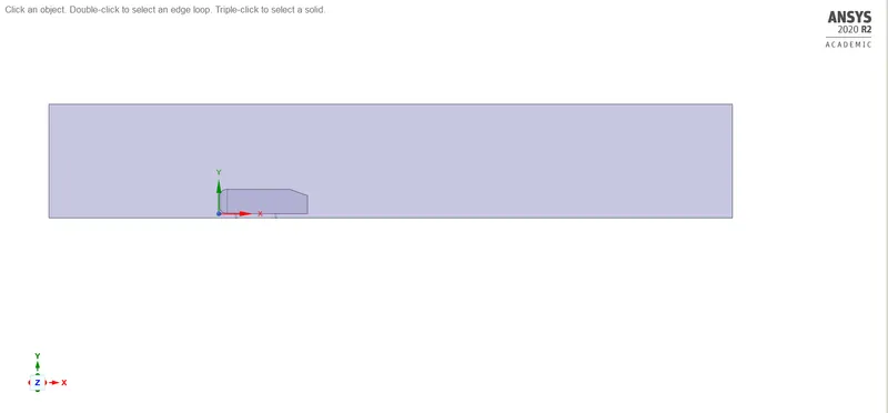
Ansys space claim is opened. A cad model of an Ahmed body is imported to the space claim. An enclosure is generated from the prepare section of the geometry. The dimensions of the enclosure is manipulated while the symetry option is turned off. The idea of bounding box or the enclosure is that the flow simulation will be studied inside the enclosure. The boundary conditions will be provided to the enclosure.

Moreover , the meshing is not required inside the Ahmed body, as it is an external body simulation. So the phsics is supressed for the Ahmed body.

When the Ahmed body is disabled or the geometry is unchecked, what the spaceclaim does is that it takes the enclosure, subtracts the volume of the Ahmed body from it and represents the same.

The dimensions of the enclosure are as follows:

Length in X direction	8.04 meters
Length in Y direction	1.338 meters
Length in Z direction	1.389 meters

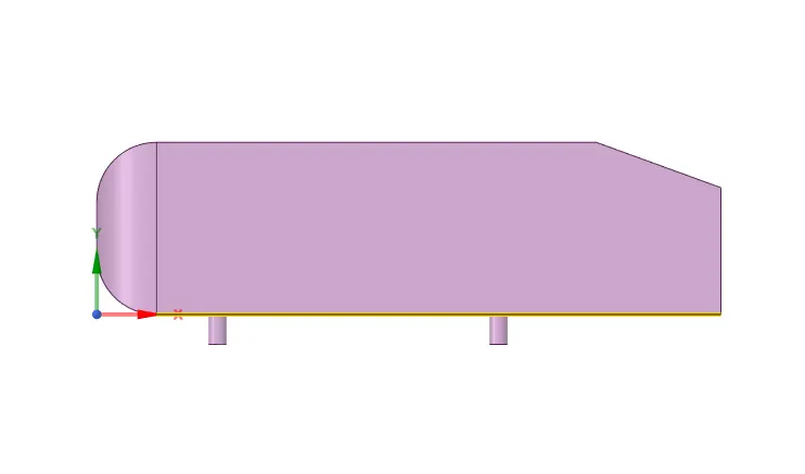
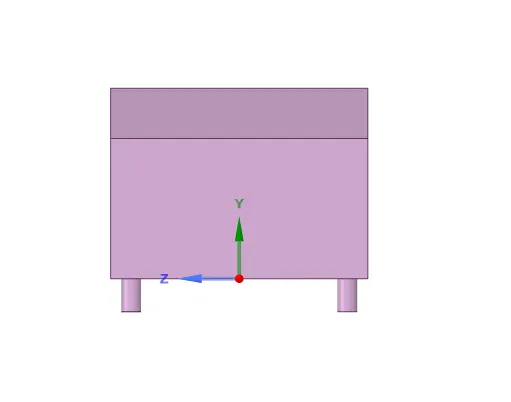
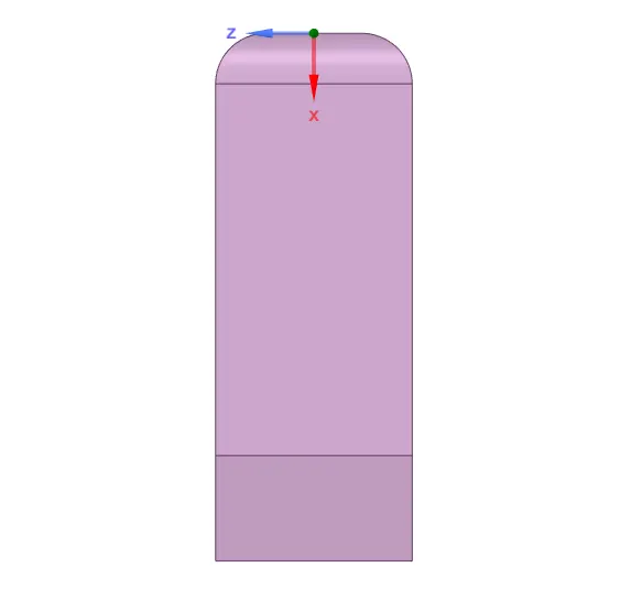
Three images above are the Ahmed body geometry along three different planes.

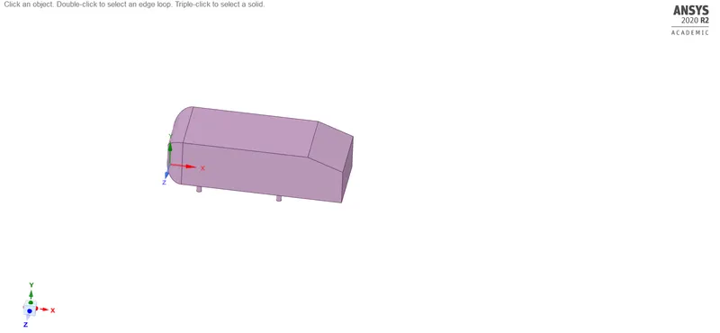
Below are the images of the ahmed body imported into the space claim and the Ahmed body inside an enclosure.

• Meshing:

As this is an baseline simulation, the default mesh that ansys generates is generated. The initial element size is 0.436 meters. the mesh is quite course but its okay for a baseline simulation.

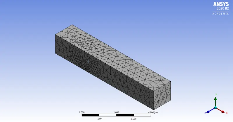
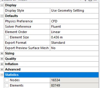
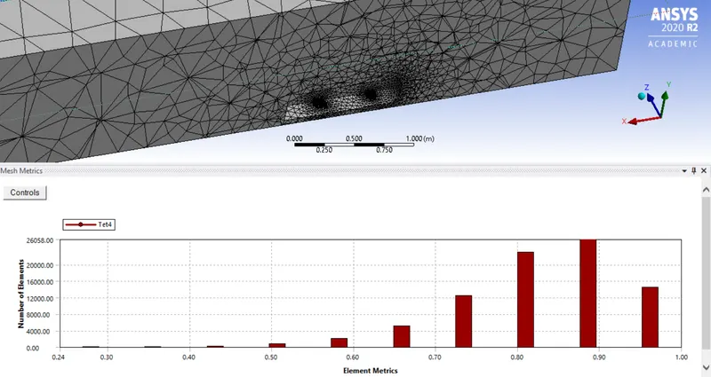
The number of elements in this case is 83749. The mesh metric shows that the mesh generated is falls in the satisfactory region. The mesh perfectly donot enters the Ahmed body as required.

Next step is the named selection. Face selection is tool is selected and the inlet, outlet, symmetry walls and the car walls are named.

• Set-up:

For the flow to be simulated, the physics of the problem needs to be defined properly. The projected area of the car walls is calculated and Fluent does an excellent jpb to by making the calculation. The refernce values are set up.

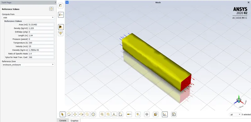
The projected area of the car walls is important as to find the coefficient of drag and lift over the same .

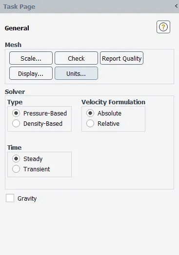
The Solver type selected is Pressure based solver as the mach number is really less. The velocity formulation is absolute ansd steady state analysis is studied.

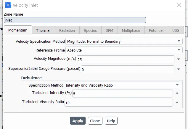
The inlet is a velocity inlet. The velocity of air at the inlet si 25 m/s. the temperature or the ambient temperature is 300 K.

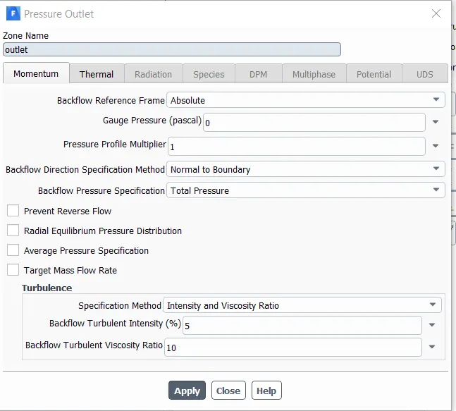
The outlet is a pressure outlet and the gauge pressure is set to 0 Pa

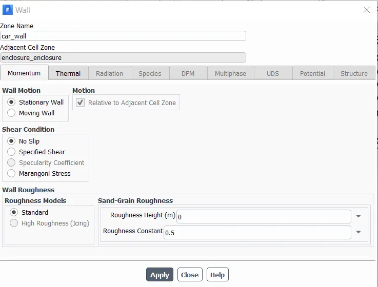
The car walls are stationary walls . No slip conditions are applied to it .

The symmetry walls have symmetry boundary conditions.

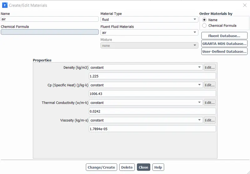
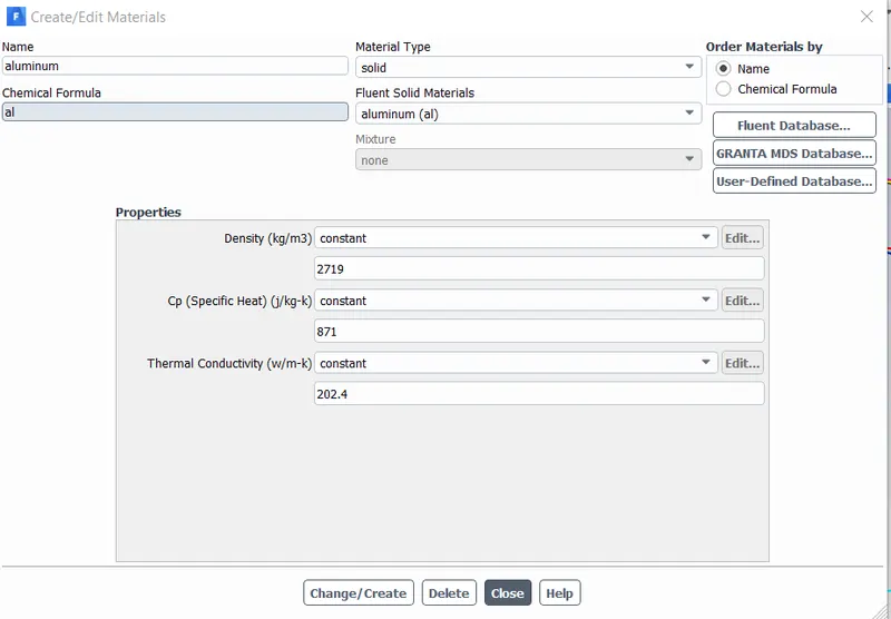
The material selected for the fluid flow is air and the Ahmed body is Almunimun.

The operating conditions are :

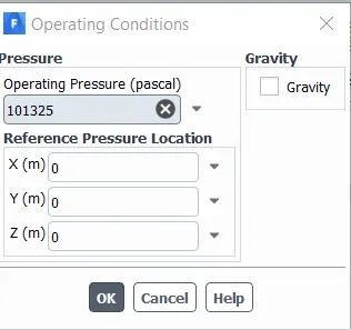Pressure = 101325 Pa , and the location of the pressure is at the origin.

The viscous model selected is K-epsilon model with standard wall functions.

The plots created for evaluation are the coefficient of drag and coefficient of lift over the car walls . The solution method selected is simple .

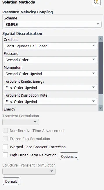The pressure calculation is second order , the momentum calcukation is second order upwind and the turbulent kinetic energy and the turbulent energy dissipation are the first order upwind.

Contors are created along a plane , for velocity and pressure for visualization of the results.

550 iterations are done .

The rsults obtained are as follows:

Co-efficient of drag	0.37
Co-efficient of lift	0.20

By comparing with the research papers , the coefficient of drag should have been 0.33.

error = 12.12%

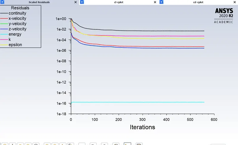
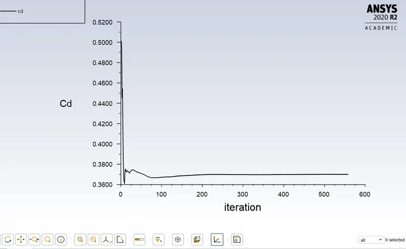
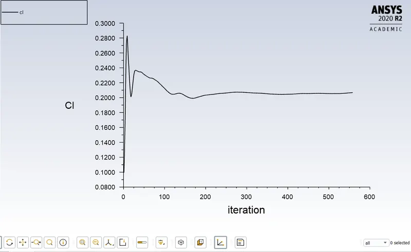
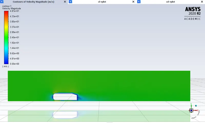
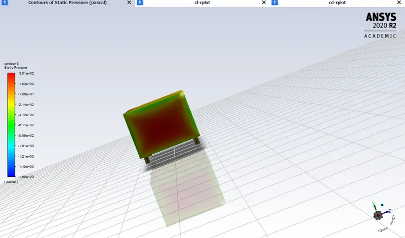
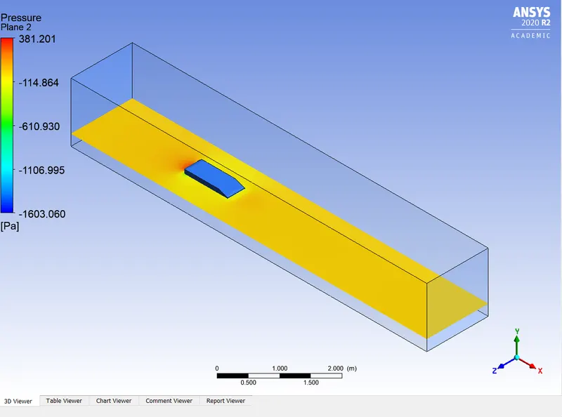
From the velocity contour along the plane , the results are really course . more refinement of mesh is required. The pressure on the car walls is shown in the second image .

• Post-Processing:

opening the CFD post, the results obtained from the simulation are visualized. A plane was created in the XY plane and the velocity and pressure contours are studied .

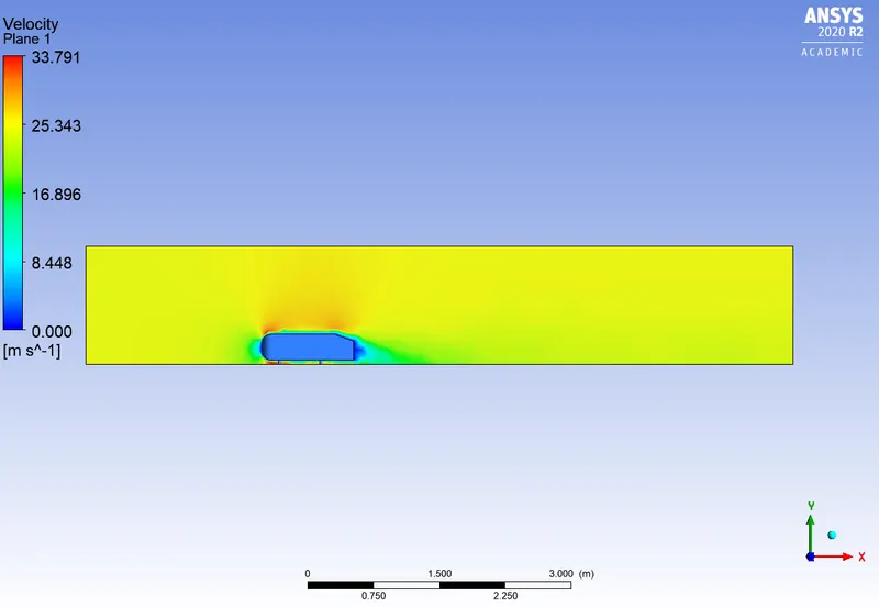
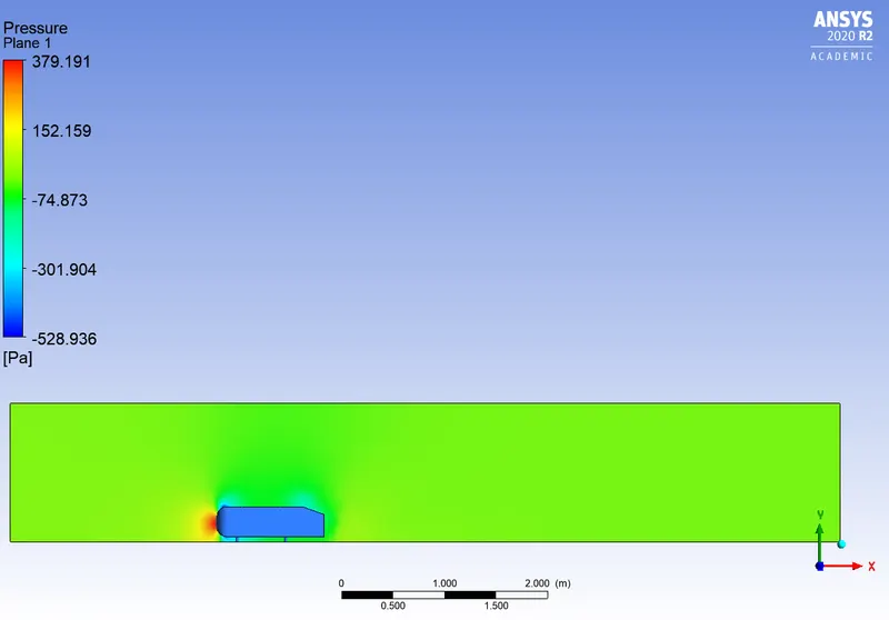
The vector plot of the velocity is as follows:

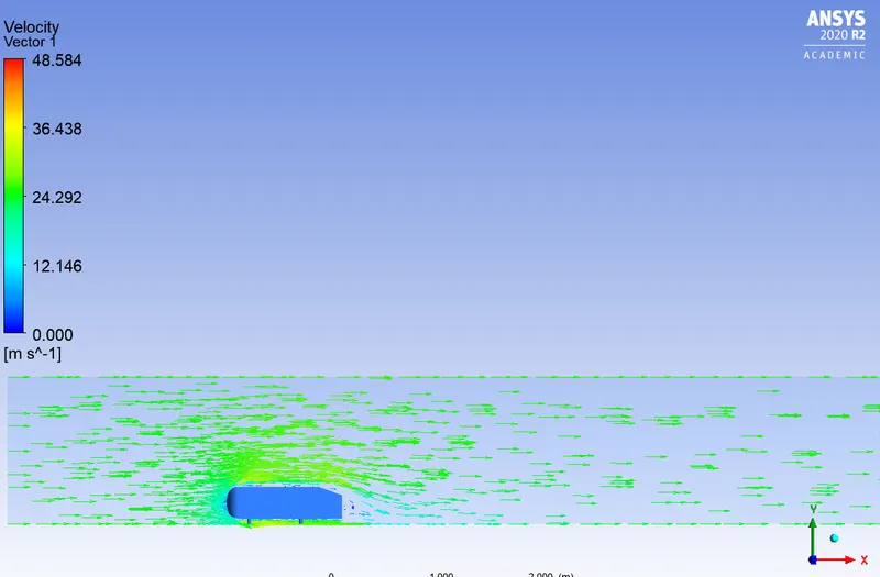
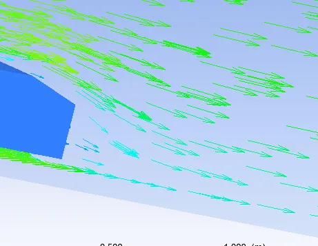
The scond image shows a zoomed on the wake region. The flow is not visualized well in this region as the mesh is course. The number of vectors in this region is way less.

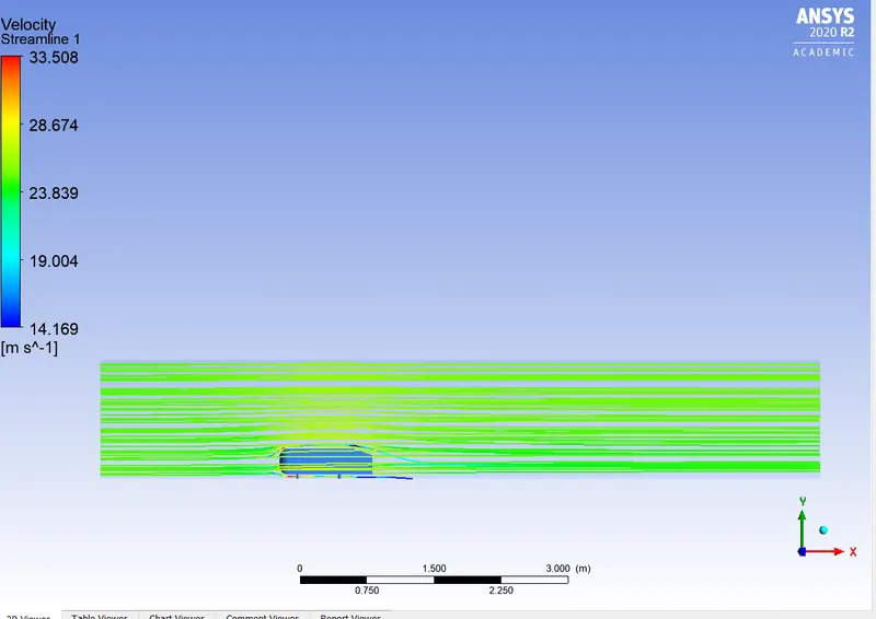
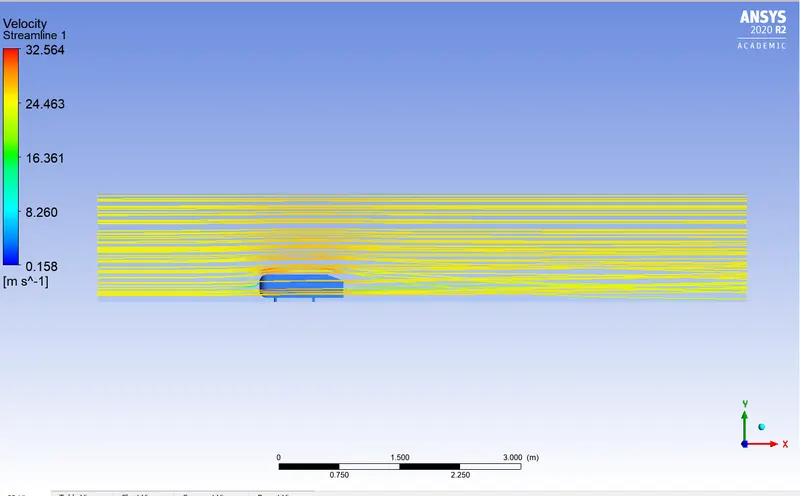
The streamlines of velocity over the Ahmed body from inlet to the outlet is :

Another plane cut in the zx plane to visulaize the pressure distributin is :

Refined Mesh simulation:

The geometry set-up is same as the previous case . Only change is in the mesh refinement.

• Meshing:

The default meshing is done. the element size is manipulated. The default elemnt size is 0.436 meters. In this case it is refined to 0.1 meters. the number of elements increases. There is a constraint in increasing the number of elements as it is a academic licence.

The mesh genereted 140550 number of elements.

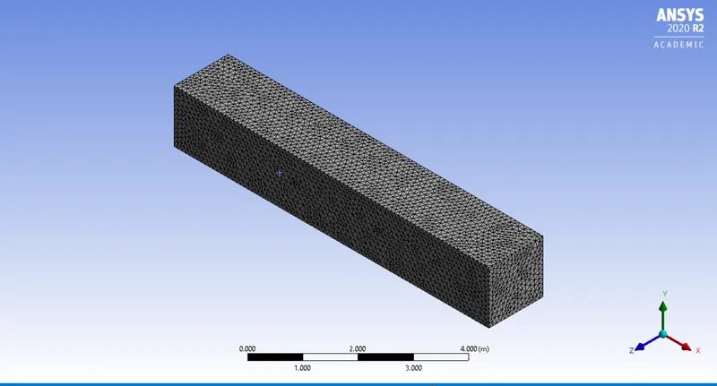
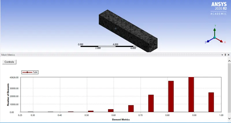
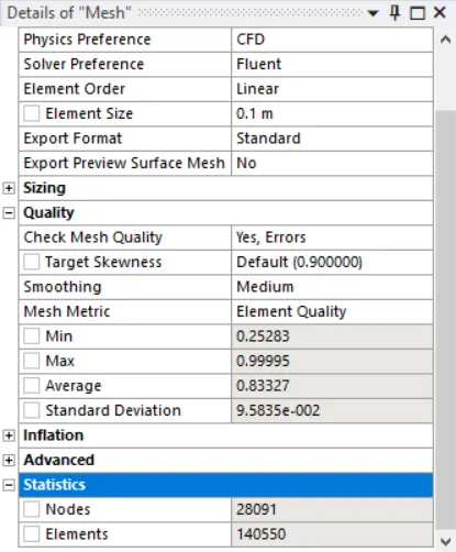
The mesh metric is satisfactory as well

• Set-up:

The model meshed is transferred to the fluent set up. All the parameters are same as the previous ones. Hybrid initialised and the 700 iterations are checked.

The scaled residual plots, coefficient of drag and coefficient of lift plots after the simulation is :

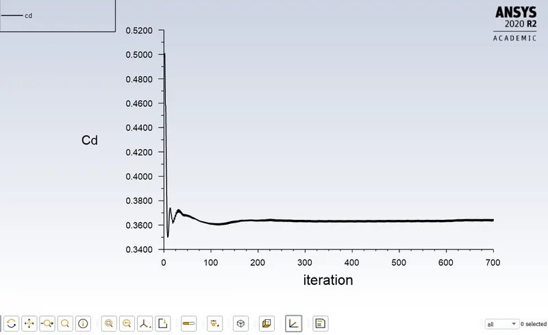
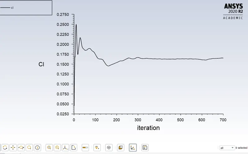
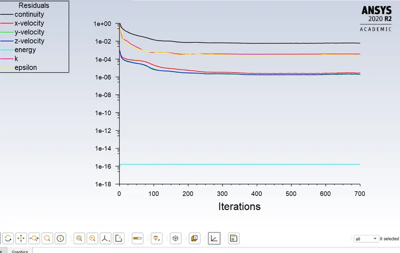
co_efficient of drag	0.3649
co-efficient of lift	0.1651

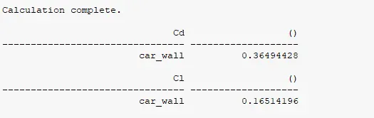
There is no major difference in the coefficient of drag value from the last simulation.

error = 9.09%

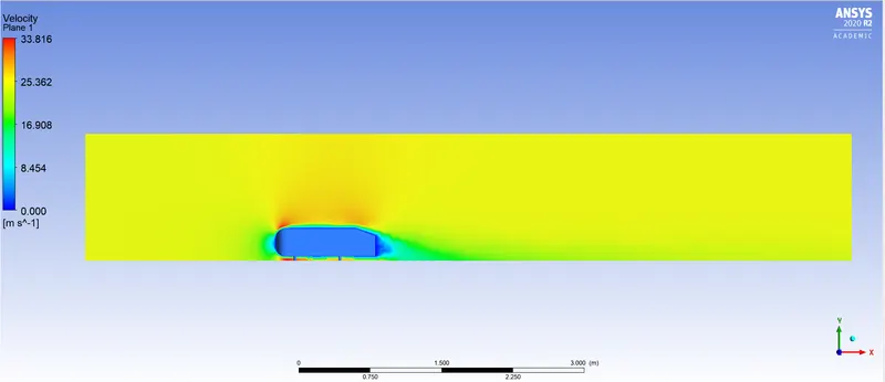
The velocity contour is :

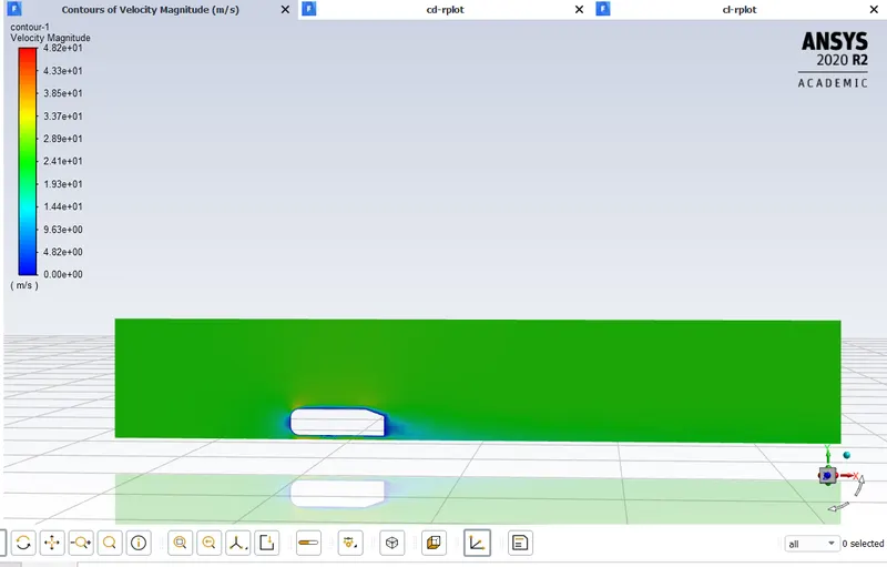
Still the wake region is diffused in nature. more refinement is required.

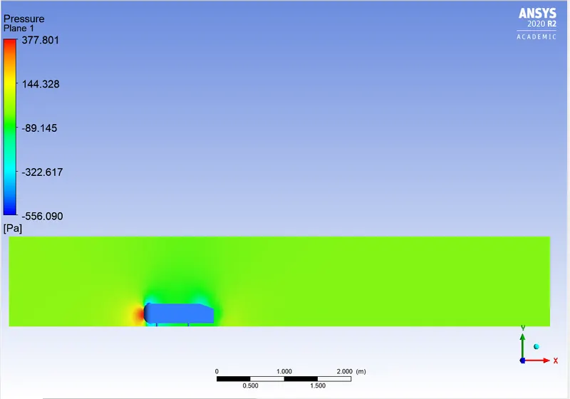
The pressure, velocity anad the streamline along the xy plane is shown below:

The vector plot is :

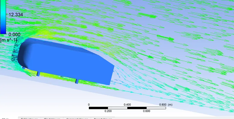
The wake region shows a less amount of vectors. refinement in the wake region of the mesh is required.

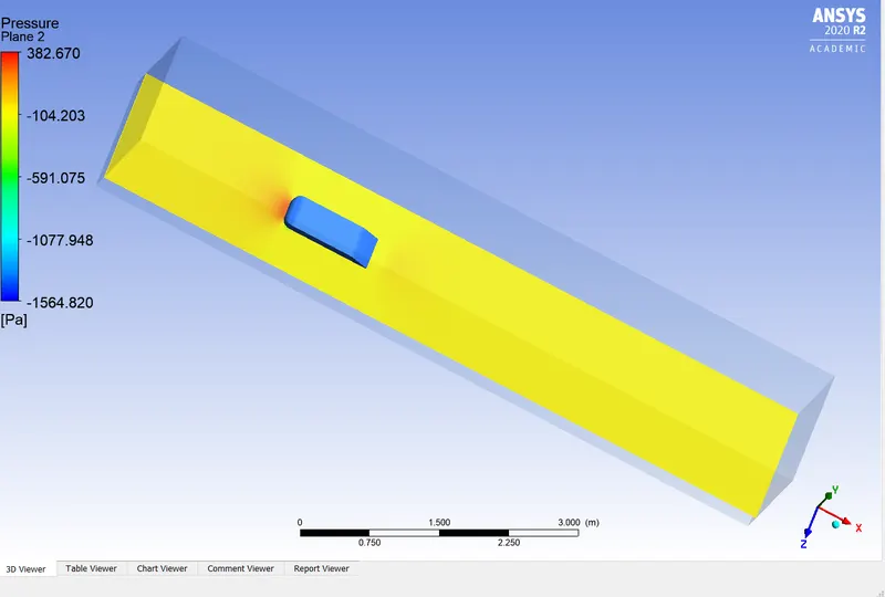
The pressure along the ZX plane is:

Refined case with Y+ modelling:

• Y-plus:

The boundary layer thickness varies with the flow parameters like reynolds number, distance from the leading edge etc. To measure a distance that scales with the boundary layer thickness we use a non dimensional parameter namely y+. In order to know where the cells are , the y+ values need to be determined so that the profile is accurate along the boundary .

`y+ = (y*uT)/(nu)`

y is the distance from the wall. nd uT is the frictional velocity.

This value of uT is determined from the reynolds number formulation.

`Re = (rho*V*L)/(mu)`

where `rho`is the density of the fluid , `V`is the flow velocity or free stream velocity . and `L`is the characteristic dimension of the body .

`V=25`

`L=1.04`

`rho=1.225`

`mu=1.78*10^-5`

calculating the Reynolds number came as 1789325.843

This is way in the turbulent region. To model the viscous sub layer region in the vicinity of the car walls, the y+ and y value is required.

skin friction coefficient `Cf=0.0576*Re^(-1/5)`

computing this the skin friction coefficient came as = 3.23*10^-3

The wall shear stress can be calculated by the formula `tau(w)=0.5*Cf*V^2*rho`

the walll shear stress value came as = 1.7805

The frictuinal velocity `u(tau)=((tau(w))/rho)^(0.5`)

`u(tau)`=1.2055

Now, the turbulence model opted for is K-epsilon with standard wall functions since its a high reynolds number problem. For standard wall functions, the y+>11. and for a K-epsilon model , y+ should be between 30 and 200.

here in this project, y+ value of 150 is aimed for. so, calculating the value of y;

y=1.80*10^-3 meters.

or 1.80 milimeters.

Now, Ansys fluent uses a Finite volume technique. FVM is a cell centroid technique. the value of y obtained is the distance of the boundary from the centroid of the first cell. So the first cell length will be twice the y value obtained.

distance of the first cell = 1.80*2 = 3.60 milimeters.

• Geometry set up:

the previous cases didnt resolve the simulation well in the wake region. In order to make the mesh finer or use local refinement . a smaller enclosure is prepared inside the lardge bounding box. symmetery option is turned off and the dimensions are created.

Interfernce is checked.

Topology is shared so that the meshing generates perfectly at the interface of two enclosures.

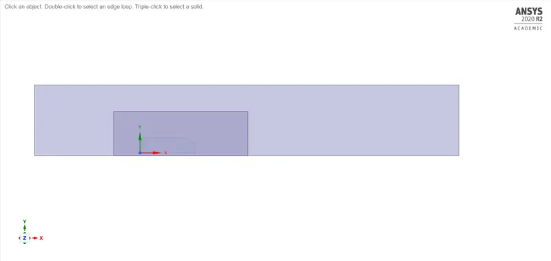
Dimensions of the small enclosures

length X	2.544 meters
length y	0.838 meters
length z	0.911 meters

• Meshing:

here local refinement is done . By selecting the body select tool and the inserting mesh methods, multizone meshing is done. The base mesh element size is 0.05 meters. The other one is hexa mesh. the maximum size is limited to 0.05 meters so that an uniform mesh is generated

Using sizing option, the car walls is meshed more finely. the element size selected for the case is 30milimeters.

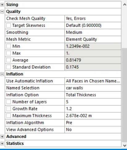
For adding inflation layers , the car walls is selected. using the option throughoout named selection inflation layers are added.

Now the first cell length should be 3.60 milimeters. here we can use the method as the first cell thickness and a growth rate of 1.2 is given for five layers. or we can use a total thickness by making necessary calculations ; having a growth rate of 1.2 and the first cell length of 3.60 meters. the total thickness to be provided is 26.78 milimeters

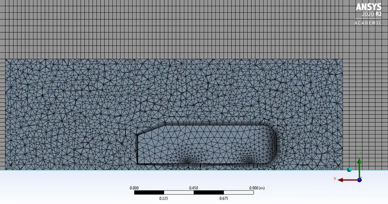
The number of elemnts in this case rose to 343169 which is below the limit

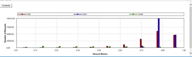
The mesh metric is :

• Set-up:

The mesh is updated and the fluent is launched. the graphics and console ischecked that all th aparameters are loaded correctly.

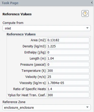
Reference values:

The values are computed from the inlet. The area is 0.13181 meter square amd length 1.04 meters. The temperature is 300 K.

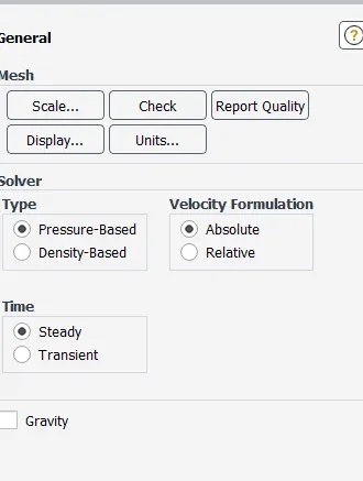
• Pressure based solver is used in the computation. Generally pressuer based solver is for low mach number flows. Mach number is defined as the ratio of velocity of fluid flow to the velocity of sound in the fluid at same conditions prevailing. velocity of fluid flow here is 25 m/s. Velocity of sound in same conditions that is 300 K is 347.18 m/s. so the Mach number comes as 0.072. For Mach number less than or equal to 0.3, the flow is considered as incompressible flow.
• Steady state analysis is done for the simulation problem
• Velocity is absolute velocity formulation.

gravity is not turned on as the anlysis is done on a horizonatal plane.

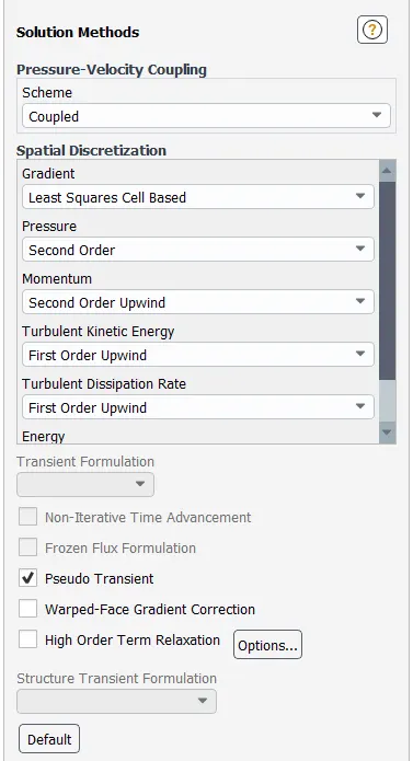
For the solution methods, a coupled scheme is selected.

Hybrid initialization is done. And the nuumber of iterations to be calcultaed is 500. The boundary conditions are same as before. The car walls are maintained at no slip condition. and the at the inlet , the air is flowed at 25 m/s . the temperature is maintained at ambient 300 K. the outket is an pressure outlet.

Coefficient of drag and coefficient of lift is plotted . Velocity and pressure contours are created at a plane.

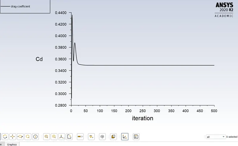
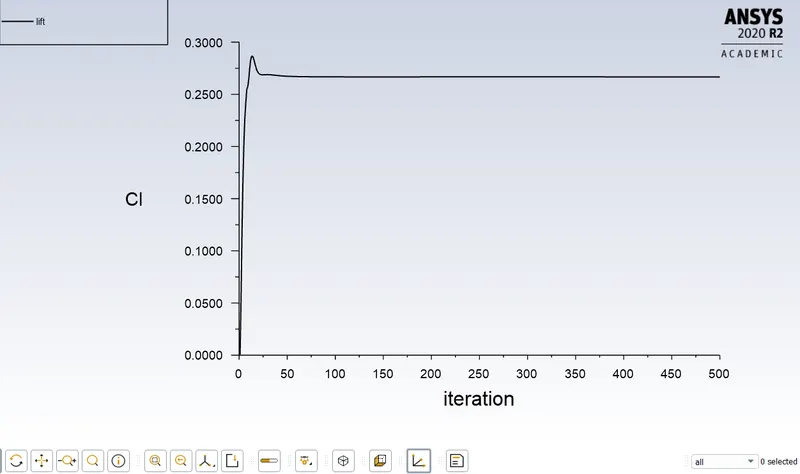
coefficient of drag	0.347
coefficient of lift	0.271

The pressure and velocity contours along the plane is:

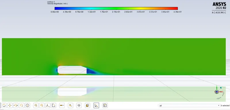
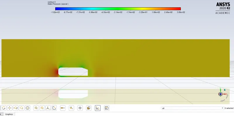
The wake region is lot more well defined now. The cofficient of drag value is lot closer to the value provided in the research paper.

error = 5.1%

The stream line along the xy plane is :

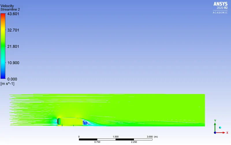
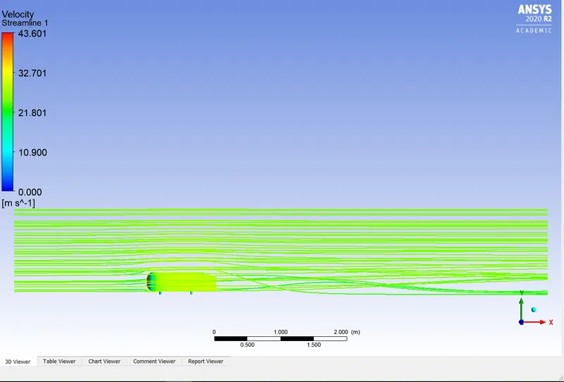
The second image is the stream line starting from the inlet of the velocity

The vector contour is :

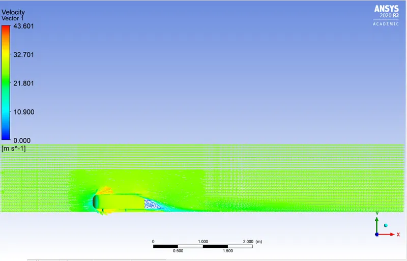
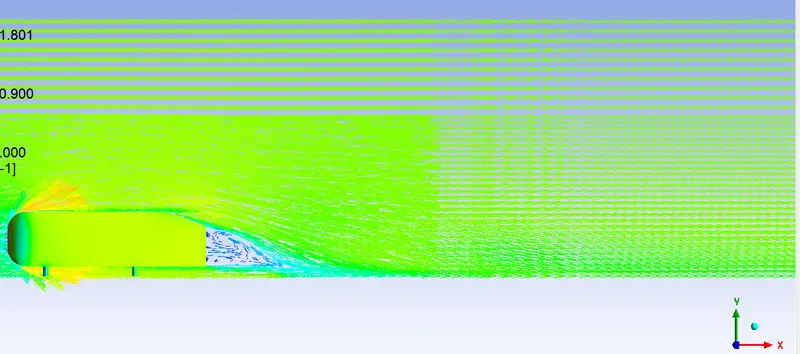
The vectors in the negative pressure region has substantially increased.

Case	Total number of cells	Coefficient of drag	Co efficient of lift
Baseline simulation	83749	0.37	0.20
Refined case	140550	0.3649	0.1651
Refined case with Y+modelling	343169	0.347	0.271

• Point of separation:

The separation pointis the point where the air stops "sticking" to an object that is moving through the air. When an object is moving through the air, the air molecules push back on it and resist the object's movement - this resistance is called pressure drag. In automobiles majority of the drag is constituted by pressure drag.

Because after the separation point the flow no longer adheres the surface of the body, the skin friction coefficient is almost zero. At the same time, however, the pressure drops considerably due to the energy dissipation in the turbulent wake. This leads to a significant increase in pressure drag, which is far greater than the reduction in skin friction drag. In total, the parasitic drag (air resistance) thus increases very strongly in the event of a flow separation.

• Negative pressure in the wake region:

The negative pressure in the wake region indicates that the lift is produced. the flow separates from the surface and creating a highly turbulent region behind the body called the wake. The pressure inside the wake region remains low as the flow separates and a net pressure force (pressure drag) is produced.

Conclusion:

The drag coefficient is reduced when the mesh is made more finer. The Velocity and the pressure contours are studied to visualize differentaspects of flow around car model. CFD codes are validated using a Ahmed Body. The set up to do a simulation on a car model is checked using a Ahmed Body

The geometry of the Ahmed body is manipulated to get drag coefficients for various slant angles . Though geometry manipulation is beyond the scope of this project.

More computational power is required to generate more finer mesh to extract exact detailing of the flow parameters.