Ahmed Body Challenge

AHMED BODY CHALLENGE

• AIM:

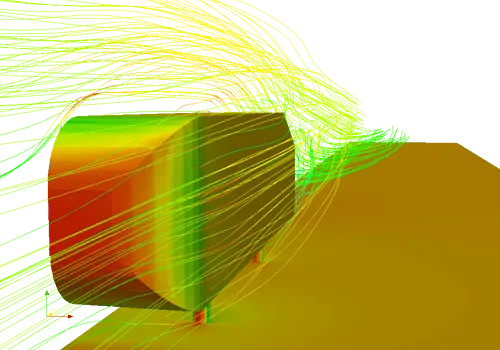
To simulate and analyse the flow over an Ahmed body with an inlet velocity of 25m/s. The shape of a car body in-front of the largest cross-section has only minor influence on the total drag. The main contributions to the drag force originate from the rear part of the body. A drag breakdown reveals that 85% of body drag is pressure drag, most of which occurs at the rear end. The rest 15% is due to friction. Thus, it is very important to design a rear body surface which brings the divided or separated streamlines smoothly together. The Ahmed body was designed with the intent to characterize this wake region that originates on the rear of an automobile. With Computational Fluid Dynamics (CFD), it is possible to visualise the flow field around the Ahmed Body.

• OBJECTIVE:

• Describe Ahmed's body and its importance.
• Explain the reason for the negative pressure in the wake region.
• Explain the significance of the point of separation.
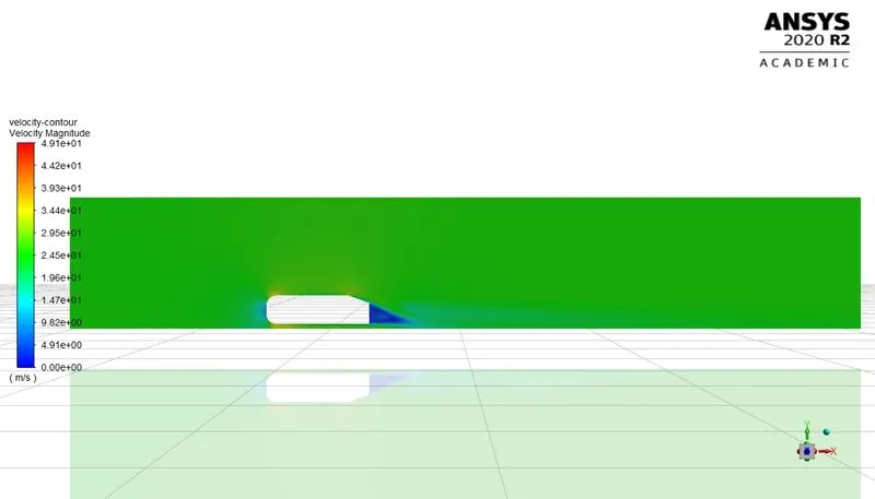
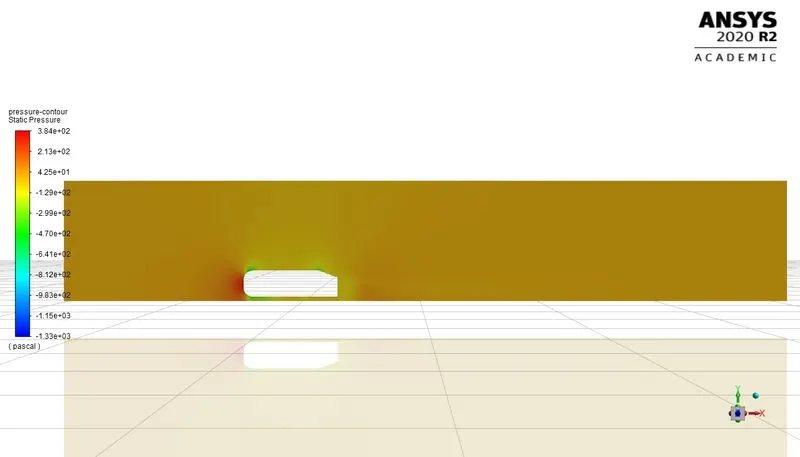
• Velocity and pressure contours.
• The drag coefficient plot for a refined case.
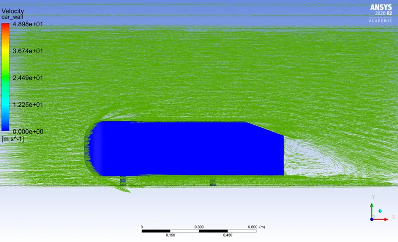
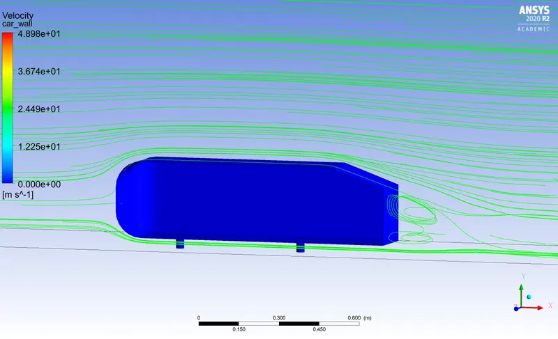
• The vector plot clearly showing the wake region.
• Perform the grid independency test and provide the values of drag and lift with each case.

• CONTENT:

• Theory:

1. Ahmed body and its importance:

The Ahmed body is a generic car body (a simplified vehicle model). The airflow around the Ahmed body captures the essential flow features around an automobile and was first defined and characterized in the experimental work of Ahmed. Although it has a very simple shape, the Ahmed body allows us to capture characteristic features that are relevant to bodies in the automobile industry. This model is also used to describe the turbulent flow field around a car-like geometry. Once the numerical model is validated, it is used to design new models of the car.

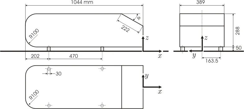
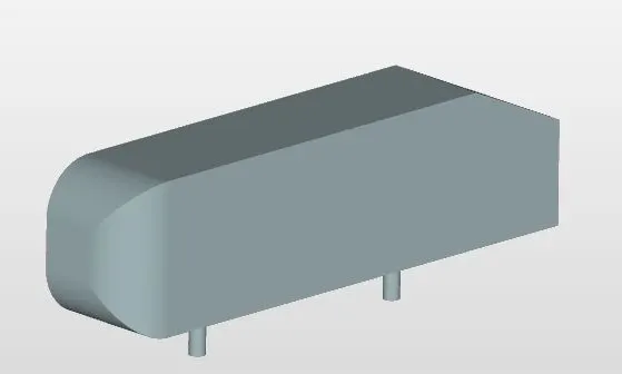
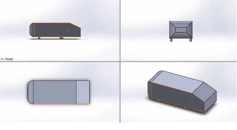
Ahmed body is simplified car model created by Ahmed et in the 1980s to investigate the behaviour of newly developed turbulence models for complex geometry cases. The Ahmed body is made up of around front part, a movable slant plane placed in the rear of the body to study the separation phenomena at different angles, and a rectangular box, which connects the front and rear slant plane as shown. Ahmed body is a simplified model of a car body, but it demonstrates all the flow features involved in an actual case of a moving car. Current vehicle development needs a strong background in aerodynamics to improve flow control by means of active or passive control devices. The complexity involved in the automobile design especially due to the great number of accessories and devices that form its geometry makes the validation tasks unaffordable. The Ahmed model is a simple geometric body that retains the main flow features, especially the vortex wake flow where most part of the drag is
concentrated and it is a good candidate to be used as a benchmark test.

The Ahmed body represents a simplified, ground vehicle geometry of a bluff body type. Its shape is simple enough to allow for accurate flow simulation but retains some important practical features relevant to automobile bodies. Selection of the configuration of this body is governed by the requirement that it should generate the essential features of a real vehicle flow field except for the flow fields that occur due to rotating wheels, engine and passenger compartment, rough underside and surface projections. The model chosen would generate strong 3-D flows in front, relatively uniform flow in the middle and a large structured wake at the rear.

2. Reason for negative pressure in the wake region:

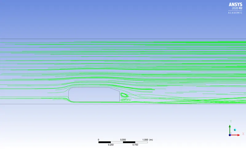
The path lines showing the exact circular motion or vorticity generation just at the rear end of the car. The separation takes two regions of distribution. One at the upper part of the rear and the other at the lower part of the rear end.

The path lines show about the nature of the fluid interaction with the rear end of the Ahmed body which here shows that the fluid just after leaving the contact from the slope still possess the momentum in it and the fluid particles near to the surface almost show the no-slip region which means the very least possible velocity of the fluid particles is in contact with the slope and base of the rear part. Thus the fluid particles away from the rear region having the higher pressure beside the wake region try to approach from the higher pressure region to the lower pressure region thus creating a circularity exactly in the wake region created.

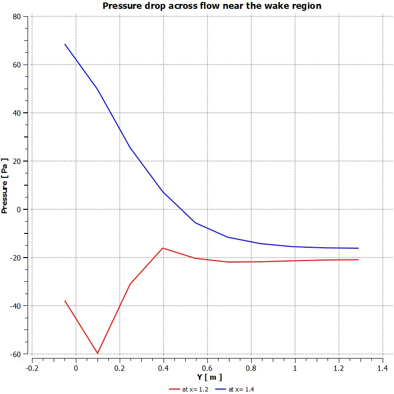
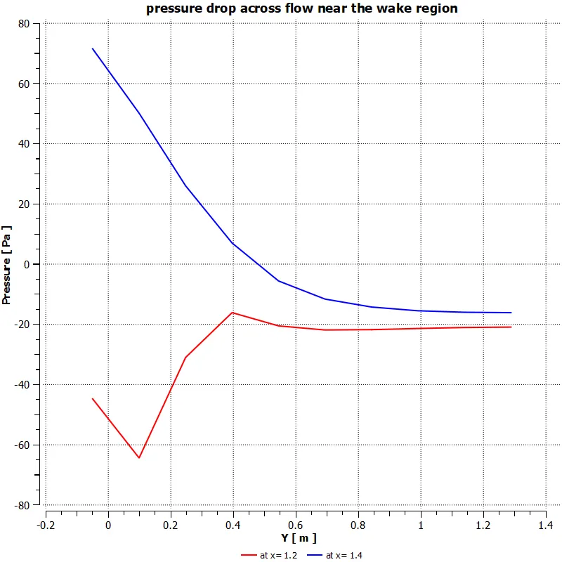
The body penetrating the fluid creates a region of emptiness just beside its end due to the nature of the geometry of the body here which can be seen least in case of a perfectly streamlined shaped body. This emptiness created is a low-pressure region towards which the fluid column exactly behind the wake region which of atmospheric pressure tries to fill the space thus dragging the fluid column with it thus creating the region of vorticity. This also results in the huge pressure gradient in the region exactly rear of the body creating the –ve pressure at the end. Also, this is the layman’s reason why there is negative gauge pressure in the wake region.

3. Significance of the point of separation:

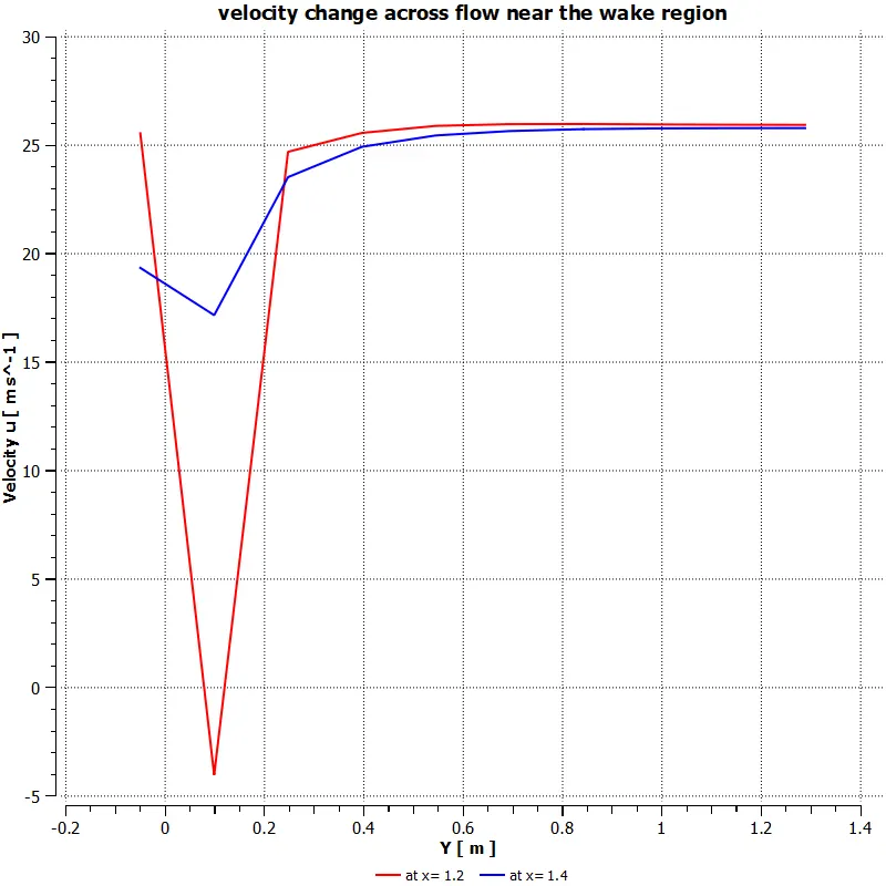
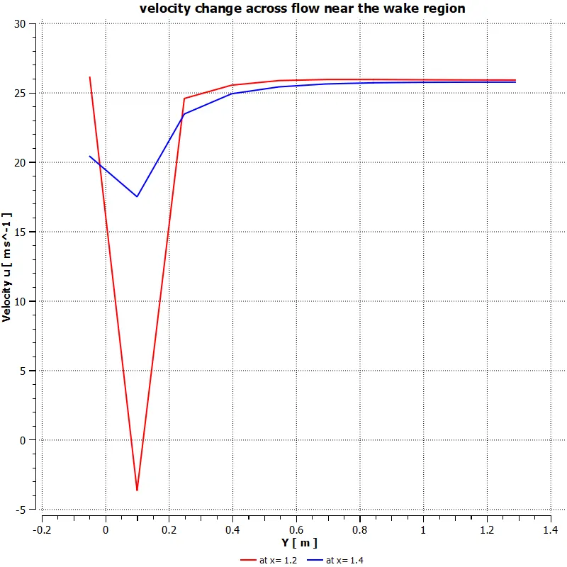
The fluid separation point can be defined as a point where the dv/dy i.e. gradient of velocity goes zero along with the dp/dx = 0, for the specific point. In more simplified term we can say that the point where the velocity gradient goes zero and the pressure gradient along the x- direction goes zero the point of separations starts occurring or the negative pressure gradient starts forming after that point. The point of separation cannot be understood just by single contour in hard and fast way. It can be supportively studied with the help of the dp/dx plots or velocity plots w.r.t the Y direction and other such plots in which we can see the nature of such physical properties like dp/dx=0, and dv/dy=0 experiencing in a particular region of fluid and body interaction.

• Geometry setup:

• Geometry setup in SpaceClaim:

As the body is perfectly symmetric, we can run the simulation by considering the only half body. This is the best practice where you can save on the number of cells and get the results faster as well. The geometry which is provided with the challenge needs a modification which you should be able to do at this stage of a course. You need to use the 'split body' command in SpaceClaim to perform the operation and then you can use the symmetry boundary condition in fluent to perform the simulation.

1. Load the Ahmed body model onto SpaceClaim and convert the units from millimetres to meters.

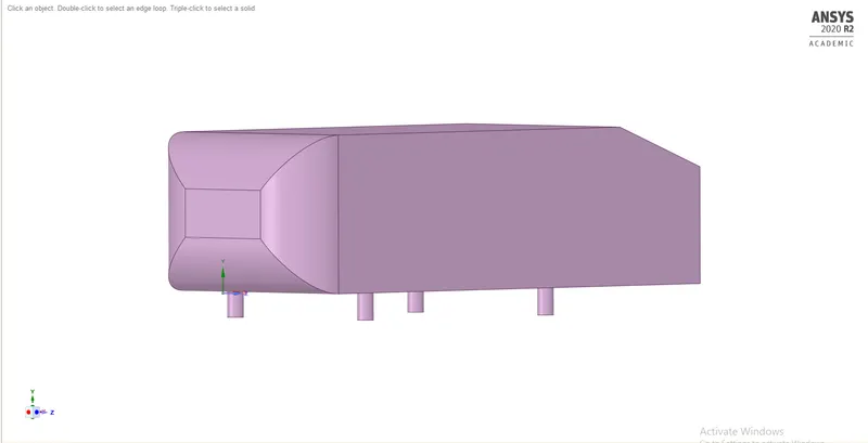
2. Go to prepare and click on the enclosure and select the Ahmed body. Enter the enclosure dimensions as per the flow requirements.

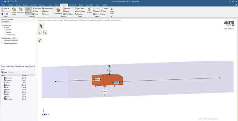
3. once the enclosure, we can create another enclosure closely around Ahmed body so that we can refine the mesh in that enclosure and still keep the total cell count less.

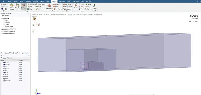
4. After both the enclosure is created, we can check interference and avoid overlapping of meshing in the 2nd enclosure by applying check interference and deleting the overlap. This is automatically done by spaceclaim when the interference option is selected inside prepare.

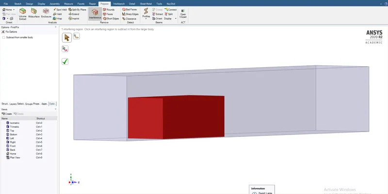
5. After clearing the interference, we can now split the body to half using the split body command in design, but before that, we have to create a XY plane at the origin to generate 2 equal halves. Select design and choose planes and bring the cursor near the origin and left-click. we get 3 planes, hide the unnecessary planes and use the XY plane.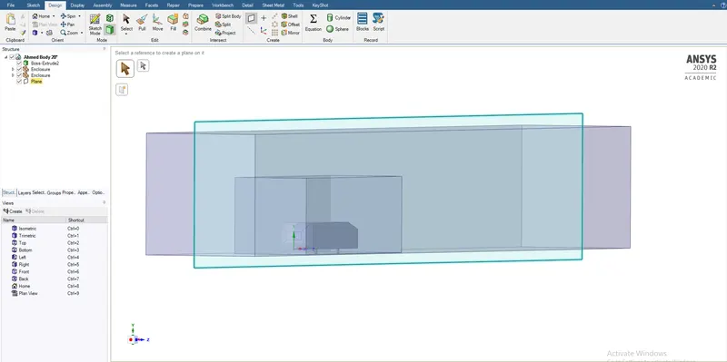

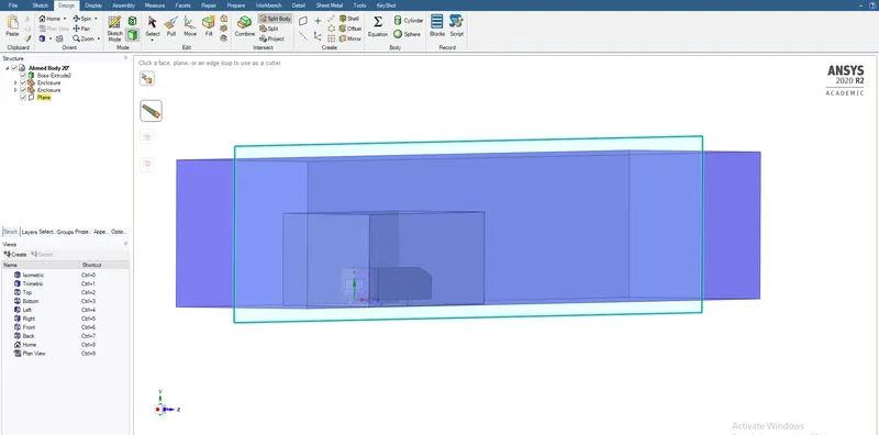
6. Now choose split body and choose the enclosure needed to split, select the plane and choose the part needed to be removed. Similarly we can achieve split on both the enclosures and the body.

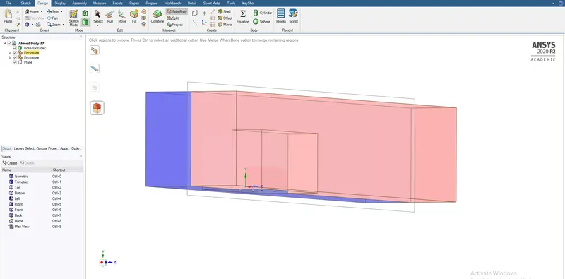
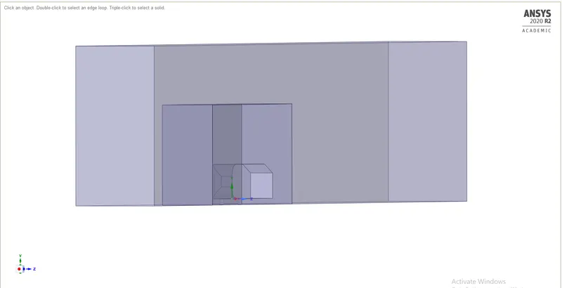
7. After achieving the split, select Ahmed body and go to properties and select Share topology. Now the mesh from both the enclosures can share the information and have a symmetry.

• Y+ and first layer wall thickness calculation:

The base grid size is chosen based on the wall-spacing values calculated by taking a desired Y+Y+ These computations are based on flat-plate boundary layer theory. The inputs required are free-stream velocity, density, characteristic length, desired Y+ and dynamic viscosity. The following equations are used to arrive at the wall spacing value:

• Reynolds Number,

`Re=(ρ⋅V⋅L)/μ`

• Skin Friction Co-efficient: It is a non-dimensional number indicating the level of friction between ahmed body and air.

`Cf=0.026/(Re)^0.142`

• Wall Shear-Stress: It is the surface shear force/unit surface and is given as

`τw=(Cf⋅ρ⋅V^2)/2`

• Friction Velocity: It gives the rate of increase of the turbulent boundary layer.

`Uf=((τw)/ρ)^0.2`

• Wall Spacing,

`y=(Y+⋅μ)/(Uf⋅ρ)`

For Y+= 70, K-epsilon turbulence model is best suited as per the theory. Wall thickness for inlet velocity of 25m/s is calculated below.

• Simulations and outputs:

constant values throughout the simulations:

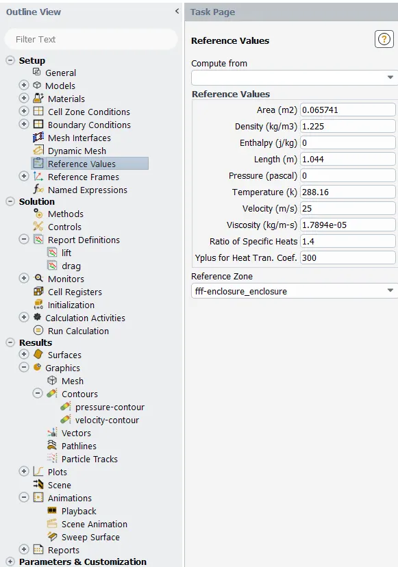
a. Reference area: 0.065741m

b. Reference length: 1.044m

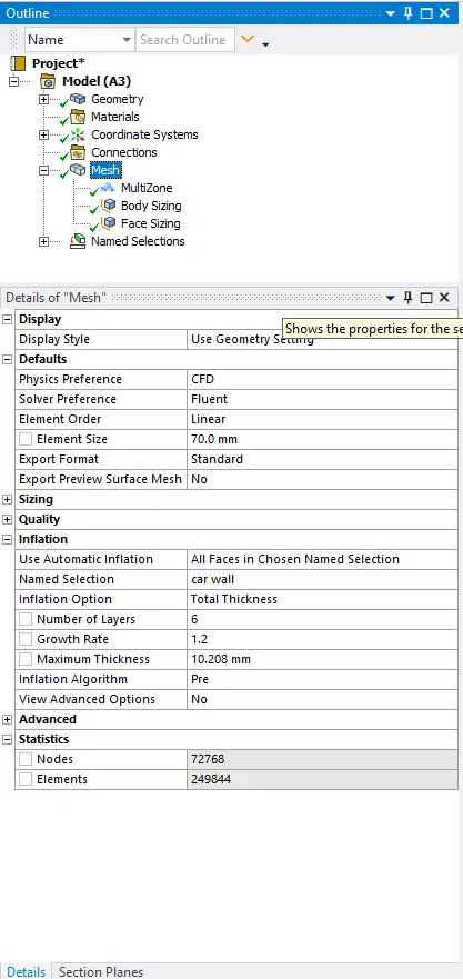
c. Inflation type and details: total thickness,

no. of layers = 6

growth rate= 1.2

Max thickness= 10.208mm

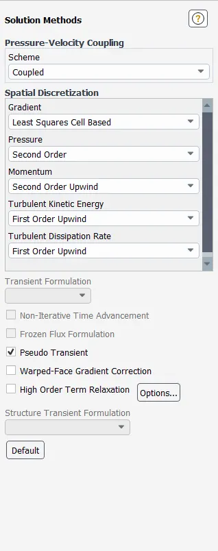
d. Pressure velocity coupling- COUPLED

• Meshing:

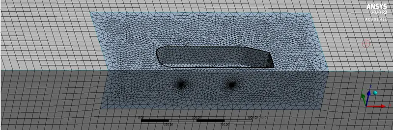
1. After creating the geometry, generate the base mesh just to check if the share topology is working correctly.

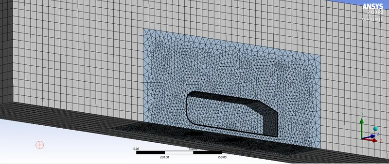
2. Click on the Inlet, outlet, symmetry wall and car wall faces separately and name the selections accordingly.

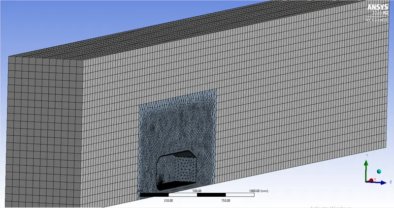
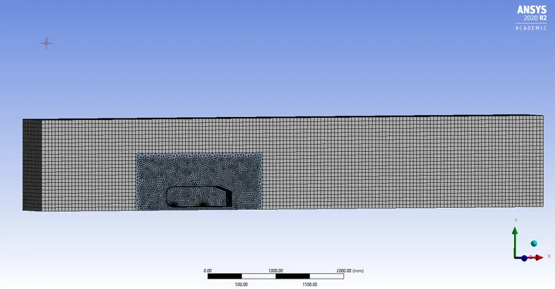
3. Right-click on mesh and choose method, click on the bigger enclosure and select the geometry and give an element size of 70mm.

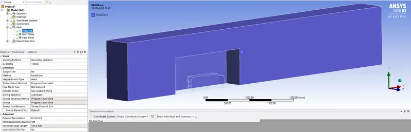
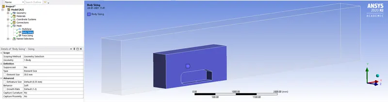
4. After generating the mesh, right-click on mesh and choose sizing. Select the smaller enclosure and give an element size of 30mm and generate the mesh.

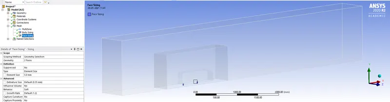
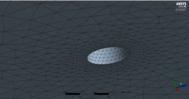
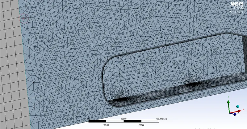
5. Choose all the faces and hit F8 so that they are hidden and now we can select the Ahmed body geometry and apply face sizing to refine the mesh near the boundary region.

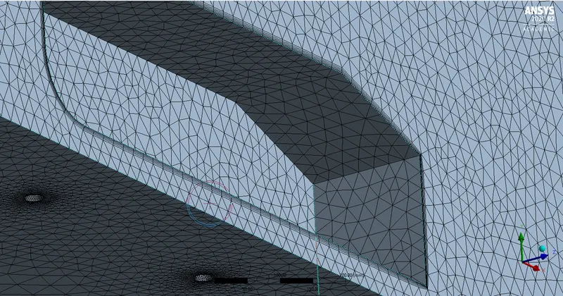
6. Click on mesh and select inflation, choose 'all name selection' at the geometry selection option. Choose total thickness method, insert the values as mentioned above at constant values section.

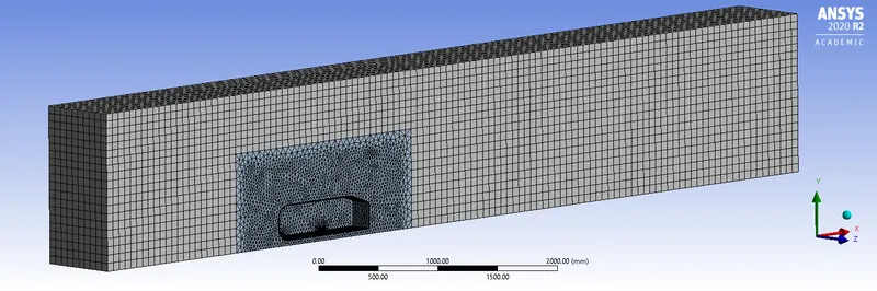
7. Close the mesh and run the fluent setup. The base mesh setup is as shown below.

• Fluent setup:

1. After setting up the mesh, choose steady-state, pressure-based solver and k-epsilon turbulence model since Y+ is greater than 30 (70).

2. Enter the reference values for the case setup and select the appropriate solution method.

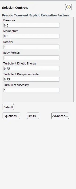
3. Calculate the Y+ value just to check if it's under the right number needed.

4. Initialise using hybrid initialisation and create contour, reports and other plots for drag and lift.

5. Choose the k-epsilon turbulence model in viscous option.

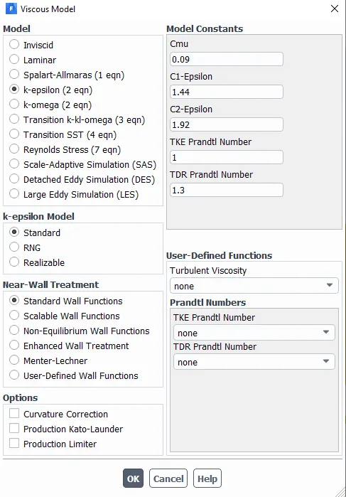
6. Check if the fluid properties are correctly initiated and taken as Air.

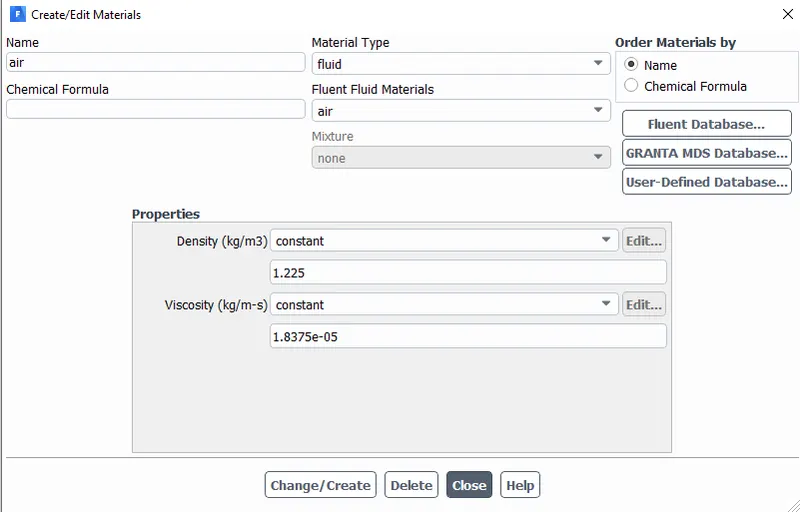
7. Check the boundary zones are correctly assigned the correct boundaries.

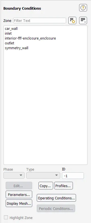
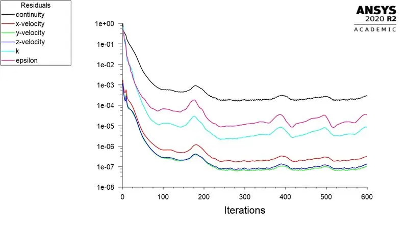
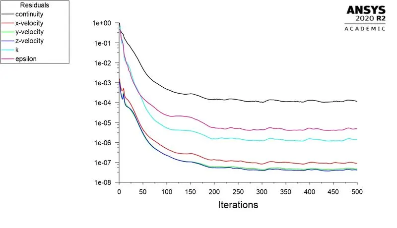
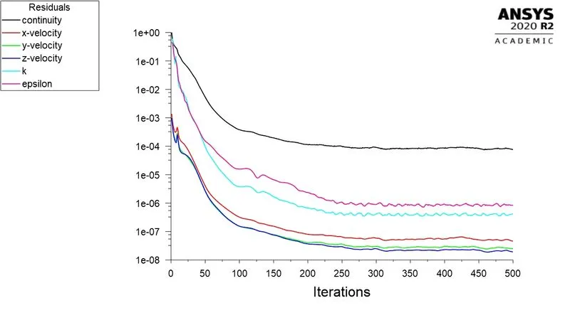
8. Run the simulation for 100 and check for convergence.

9. If the simulation is stable and simulating correctly, run the simulation for 600-700 iterations to reach convergence.

• CFD post:

1. After the fluent has run the simulation, we can close fluent and open results to work on post-processing using CFD post.

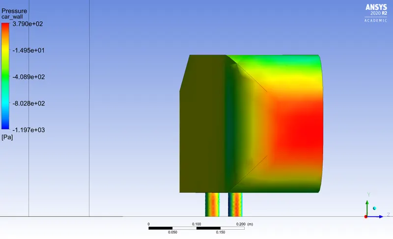
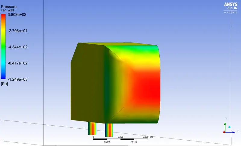
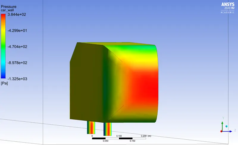
2. Tick on car wall to display the car wall, double click and change from constant to variable and choose pressure and click apply to view the amount of pressure acting the car body.

3. Create a cut plan normal to z-axis by clicking insert, plane and create. Under domain, use variable and select velocity and click apply.

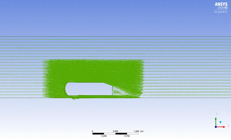
4. Create vector plane by choosing vector under insert and under the domain, choose a variable under the domain and choose velocity to view the vector lines along the flow and understanding the flow near the wake region.

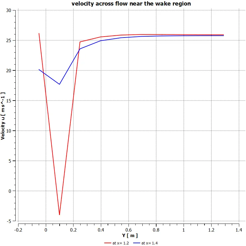
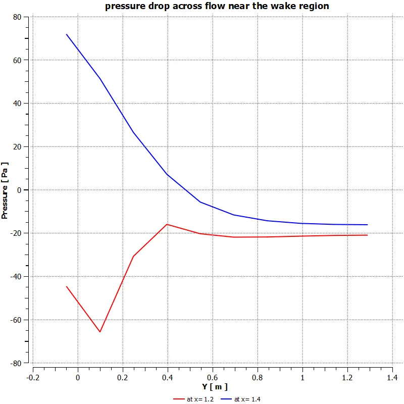
5. Create a line near the wake region by using insert and choose line, and use chart option to plot the info of velocity and pressure flowing across that line.

• Results:

1. Base Mesh:

a. Total elements: 249844

b. Main Mesh (enclosure 1): 70 mm

c. Body sizing (enclosure 2): 30 mm

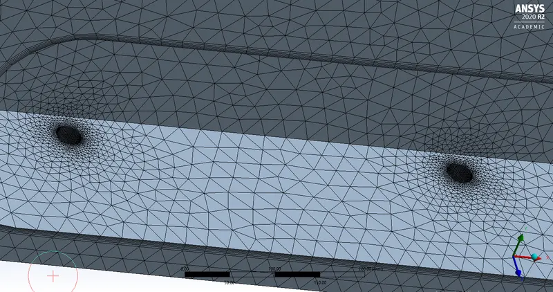
d. Face sizing(refining the cylindrical stands) = 5 mm

• Mesh:

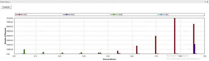
• Mesh quality:

• Plots and Contours:

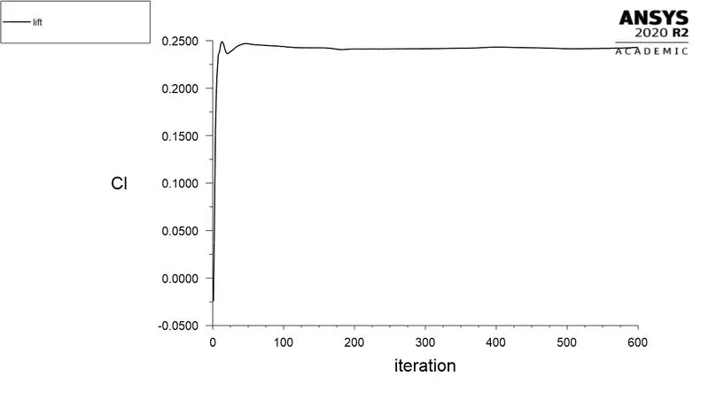
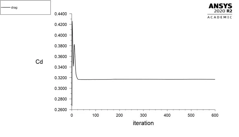
1. Lift and drag plot:

2. Velocity and pressure contours:

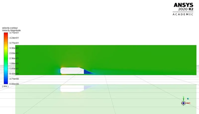
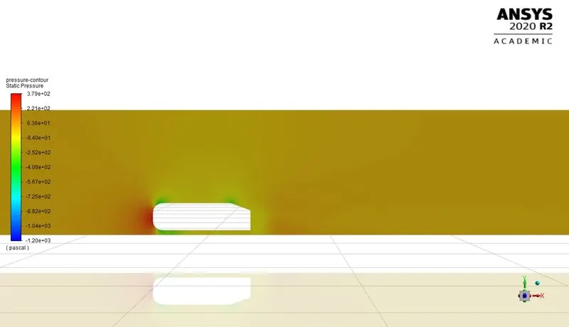
3. Velocity vector and streamline plot:

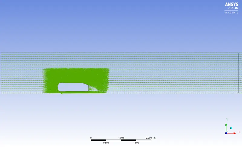
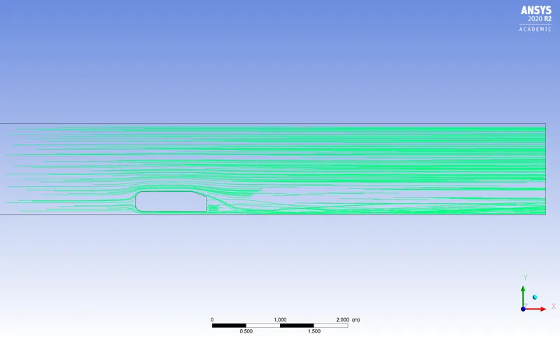
4. Residuals and pressure acting on the car wall:

5. Velocity and pressure change across the flow:

2. Refined Mesh:

case 1:

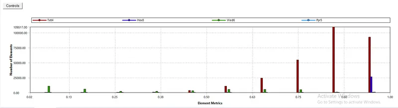
a. Total elements: 356998

b. Main Mesh (enclosure 1): 65 mm

c. Body sizing (enclosure 2): 27 mm

d. Face sizing(refining the cylindrical stands) = 3 mm

• Mesh:

• Mesh quality:

• Plots and contours:

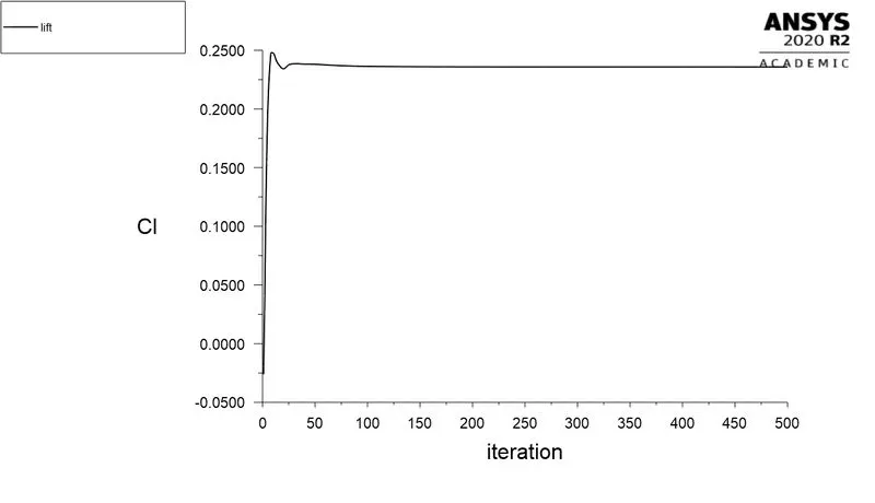
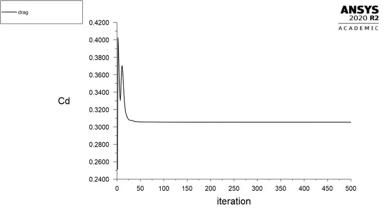
1. lift and drag:

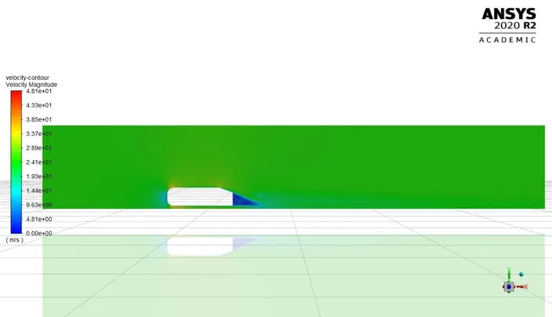
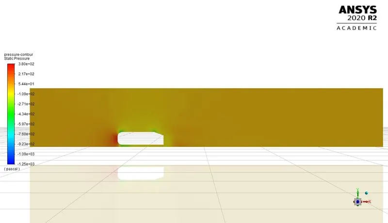
2. Velocity and Pressure contours:

3. Velocity vector and streamline:

4. Residuals and pressure acting on the car wall:

5. Velocity and pressure change across the flow near the wake region:

case 2:

a. Total elements: 493898

b. Main Mesh (enclosure 1): 55 mm

c. Body sizing (enclosure 2): 25.8 mm

d. Face sizing(refining the cylindrical stands) = 1.6 mm

• Mesh:

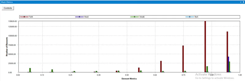
• Mesh quality

• Plots and contours:

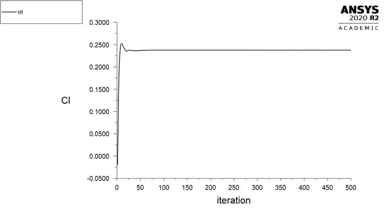
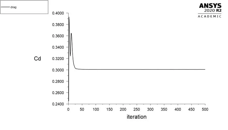
1. Lift and drag plots:

2. Velocity and pressure contours:

3. Velocity vector and streamline:

4. Residuals and Pressure acting on the car wall:

5. Velocity and pressure change across the flow near the wake region:

• CONCLUSION:

Table showing drag and lift coefficients for each grid independency test.

Mesh Size	No. of Elements	Cd	Cl	Error %
Base Mesh size 70mm Inner body size = 30mm	249844	0.3167	0.2430	2.67
Mid refined Mesh size 65mm Inner body size = 27mm	356998	0.305	0.235	1.5
Refined Mesh size 55mm Inner body size = 25.8mm	493898	0.3007	0.224	1.07

Inference from the above table:

From the above table with the refinement of the mesh drag coefficient approaches closer to the analytical values that are because more cells are assigned at the boundary layer which results in more accurate results of drag coefficients.

Conclusion:

1. High pressure is formed at the frontal area of the Ahmed body due to loss of kinetic energy of the air.
2. The adverse pressure gradient is created near the wake regions because of the flow separation which is occurring because of the geometry of the model. As a result flow separation alters the pressure gradient which in turn affects the drag and lift coefficients.
3. In order to reduce the size of the wake region, detachment of the fluid should be farther away from the body which can be achieved by an increase in the slant angle.
4. With the decrease in mesh size, the numerical results approach closer to experimental results.