Ahmed Body Challenge
Problem Definition
1.Perform the simulation on half of Ahmed's body (perfectly symmetric) to plot the velocity and pressure contour.
2. Calculate and plot the drag and lift coefficient.
3. Plot the vector plot showing the wake region.
Introduction
Ahmed's body
The Ahmed body is a generic car body (a simplified vehicle model). The airflow around the Ahmed body captures the essential flow features around an automobile and was first defined and characterized in the experimental work of Ahmed. Although it has a very simple shape, Ahmed's body allows us to capture aerodynamic features that are relevant to bodies in the automobile industry.
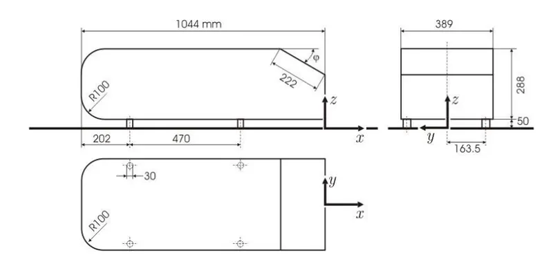
The flow region which presents the major contribution to a car’s drag, and which poses severe problems to numerical predictions and experimental studies as well, is the wake flow behind the car. The location at which the flow separates determines the size of the separation zone, and consequently the drag force.
A more exact simulation of the wake flow and of the separation process are essential for the correctness of drag predictions. However, a real-life automobile is a very complex shape to model or to study experimentally. Therefore the MOVA consortium partners agreed to study the vehicle shape employed by Ahmed, known as the Ahmed body.
So when we are simulating the in CFD to calculate the experimental data to observe the behaviour of turbulence and pressure, we are going to validate our data with Ahmed's body model data. Ahmed body is a simplified bluff body which maintains the accuracy when we are modelling air-flow around the vehicle while maintaining the features of the vehicle. So Ahmed body is a successful model which gives us good predictions of the separation process and wake flow.
So we are going to simulate Ahmed's body and going to check what will be going to the drag and lift coefficient and what is happening in the wake region. We are going to check the effect of pressure and velocity in the wake region.
Drag Force
A drag force is the resistance force caused by the motion of a body through a fluid, such as water or air. A drag force acts opposite to the direction of the oncoming flow velocity. This is the relative velocity between the body and the fluid.
Drag Coefficient
The drag coefficient(`C_d`) is a dimensionless quantity that is used to quantify the drag or resistance of an object in a fluid environment. The Drag coefficient is given as:
`C_d = (2*F_d)/(rho*u^2*A)`
where
`F_d` = drag Force (N)
`rho` = density of the fluid (kg/`m^3`)
u = Flow velocity (`ms^-1`)
A = cross-sectional area (`m^2`)
Lift Force
A fluid flowing around the surface of an object exerts a force on it. Lift is the component of this force that is perpendicular to the oncoming flow direction. Lift is a mechanical force. It is generated by the interaction and contact of a solid body with a fluid (liquid or gas). It is not generated by a force field. Lift is generated by the difference in velocity between the solid object and the fluid.
Lift Coefficient
The lift coefficient (CL) is a dimensionless coefficient that relates the lift generated by a lifting body to the fluid density around the body. It is used to determine the lift of an object in a fluid environment.
`C_L = (2*F_L)/(rho*u^2*A)`
where
`F_L` = drag Force (N)
`rho` = density of the fluid (kg/`m^3`)
u = Flow velocity (`ms^-1`)
A = cross-sectional area (`m^2`)
Assumption
In this case, we have the following assumption
1. The inlet velocity of the fluid is 25 m/s.
2. We have to use default air properties.
Case setup
1. First we are going to open the workbench and going to click on the Fluid Flow(Fluent). It is going to open the module in the Project Schematic.
2. Now we are going to click on the geometry. It will take you to the spaceClaim. Here we are going to open the existing design.
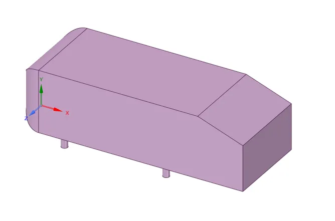
3. Now we are going to create an enclosure surrounding this body. So for that we are going to choose the Enclosure option in Prepare and we are going to select the body and we are going to give the measurement to that enclosure. We are going to prepare two enclosures to Ahmed's body.
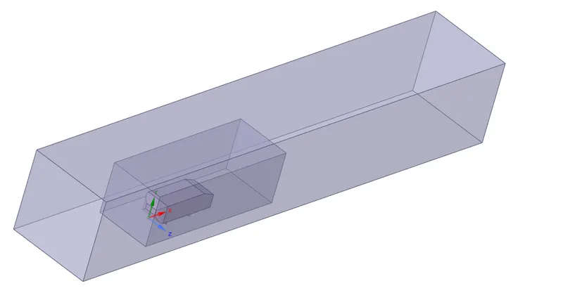
4. Now we are going to cut the body in half with the 'split body' command. Now we are going to close the spaceClaim.
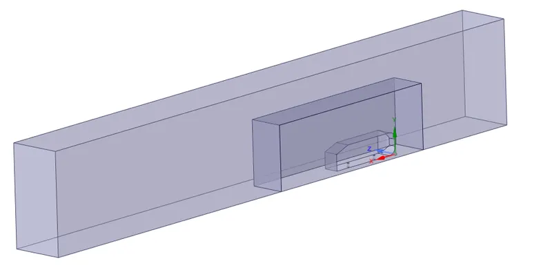
5. Now we are going to click on the mesh. It will take us into the meshing. Here we decide what mesh element size we are going to take and we are going to give the inlet, outlet, symmetry-name and car-wall name to the face.
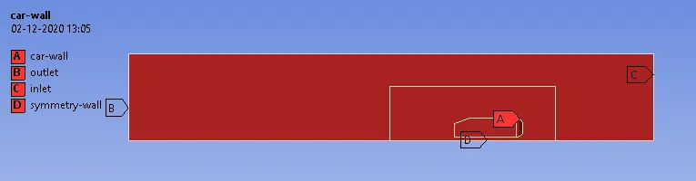
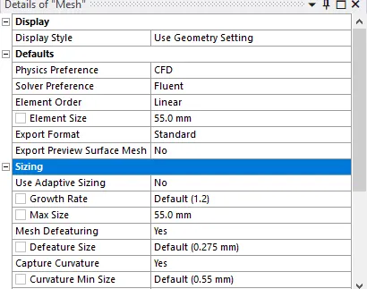
6. Now we are going to give the mesh element size to make the mesh finer. We are going to give the element size to the outer domain and maximum element size to be exact as the mesh size.
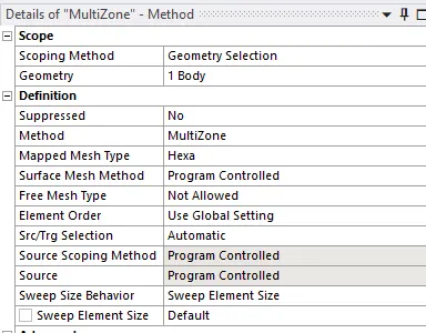
Now we want that outer body has the hexagonal shape elements so we are going to insert the method and we are going to give mesh type to be Hexa.
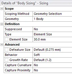
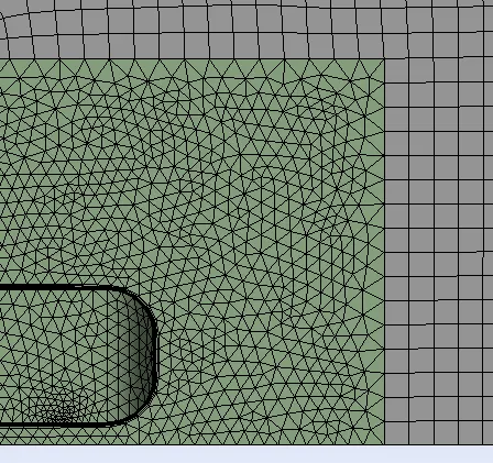
Now we are going to give the mesh size to the body and we are going to take the element size to be smaller than the domain element size.
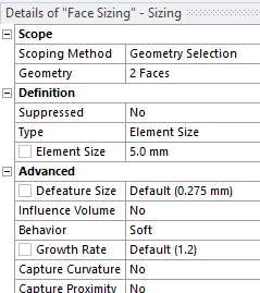
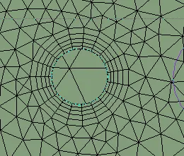
But we can see that the circle is not the proper shape so to make it more smooth we are going to give a very small element size to that part.
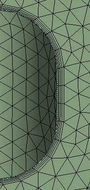
Now we are going to make the inflation layer to capture the boundary layer properly. So I have taken the 5 inflation layer with a total thickness of 12.5 mm with a 1.2 growth rate.

Now we are going to generate the mesh.
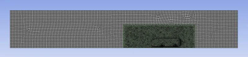
outer domain and body mesh
inflation layer
face sizing
7. Now we are going to update the mesh and then setup. Now we are going to open the setup it will take us to the Fluent. Here we are going to setup our case. So we are solving the 3-D problem. We are going to use double precision and we are going to use 4 Solver Processes(parallel). So now when we start it will take us to the Fluent.
8. In the Fluent we will go to Physics. Here we choose the type of solver, we have taken the pressure-based type solver. Now we have to choose the velocity formulation, we have taken absolute velocity formulation. Now we are going to choose the time solver, we are using a steady time solver.
9. The flow is turbulent so we are going to choose the `k-epsilon` or `k-omega` module to solve this problem. I have simulated with both models and the result are more accurate when I used the `k-omega` SST model. So that's why I am going to show you the result with the `k-omega` model.
10. Now we are going to choose the material. We have taken the air as the material and we are going to choose the default values.
11. Now we are going to give the boundary condition:-
So we are giving the velocity inlet v = 25 m/s
Pressure outlet (Gauge pressure) = 0 Pa
12. Now we are going to click on the solution. Here we are going to create the definitions. We want the drag force coefficient and lift coefficient.
13. Now we are going to initialize the solution and we are going to create the pressure and velocity contour. And we have to change the value in the reference which is present in the result section in reports.
14. Now we are going to simulate the result and we will get the plots and results.
Results
Residual
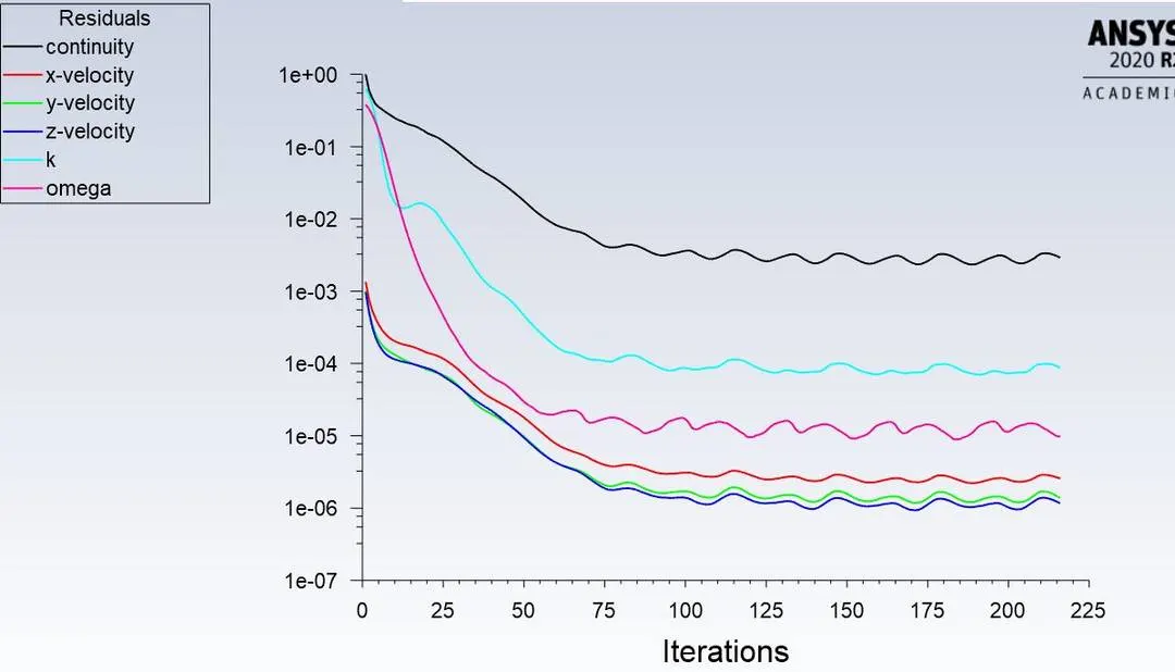
So from the residual graph, we can see that after some iteration the plot is repeating the same pattern. So we can say that the result got converged and we get the steady-state condition.
Drag Coefficient
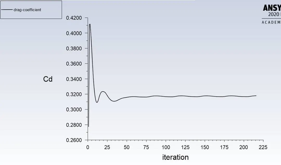
We can see that the graph is repeating the same pattern after some iteration so we get the converged value. The drag coefficient we get is 0.3179.
Lift Coefficient
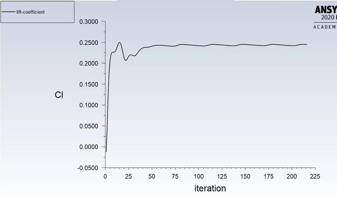
We can see that the graph is repeating the same pattern after some iteration so we get the converged value. The lift coefficient we get is 0.2449.
Pressure Contour
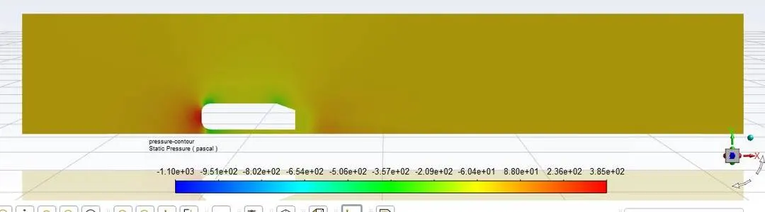
In the above figure, we can see that the pressure distribution in the entire domain.
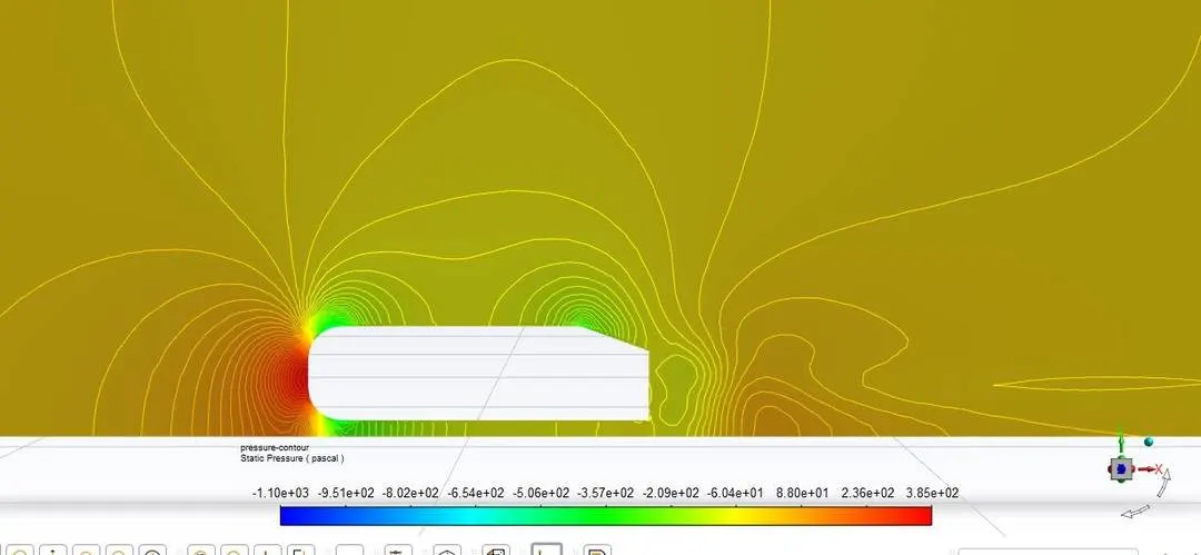
So we can see from the graph that at the inlet of Ahmed body pressure is higher.
Velocity Contour
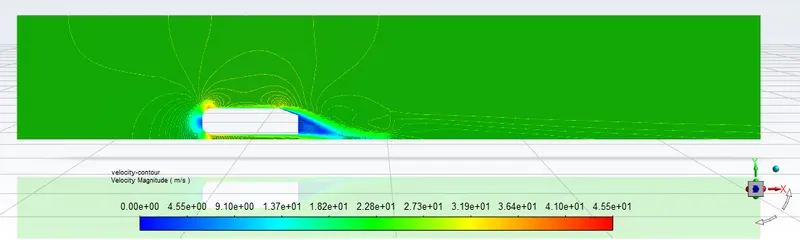
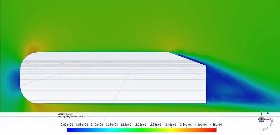
We can see from the contour that how is the velocity distribution in the domain. We are getting the velocity to be zero at the end of Ahmed's body that is the wake region.
Path line of velocity
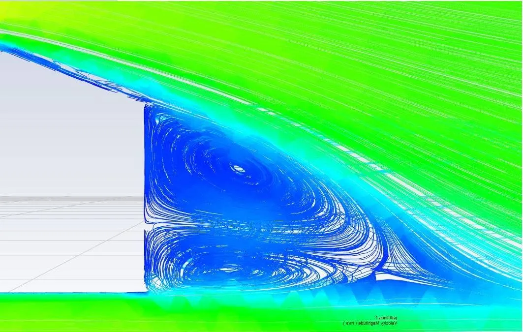
In the path line velocity contour, we can see that there are two eddies are forming at the end of Ahmed's body. The path lines showing the circular motion of the air at the rear end of the car. There are two eddies are forming. One at the upper part and the other at the lower part at end of the body.
Vector plot
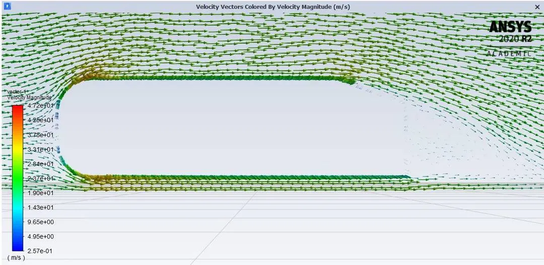
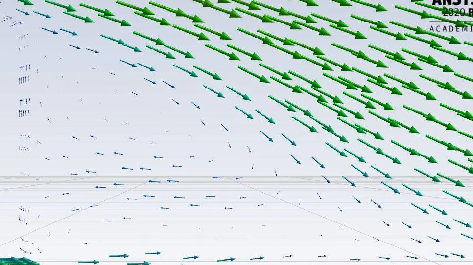
This is the vector plot in which we can see how the air is flowing around Ahmed's body. We can see that at the wake region air is in very small amount.
Inference
The velocity of the air decreases suddenly at the front of Ahmed body because when the air hits the front area of the body it generates kinetic energy and pressure increases. Because of that, the air goes to the low-pressure region. So the air will be going to the top of the body because fluid always flows from the high pressure to the low pressure region.
As the air goes to the rear end at a point there is a sudden geometry change because of that wake region generated.
Wake region creates because of the slant edge it leads to creating the vacuum at the end of the body. So because of the vacuum, there will be no air and we will get the pressure to be negative.
So if the wake region is large the eddies will be larger which is bad. Because it creates pressure disturbance in the flow that we don't want. So to get the smaller wake region the point of separation should be at the end of the body as posible.
Grid Independence
Case-2
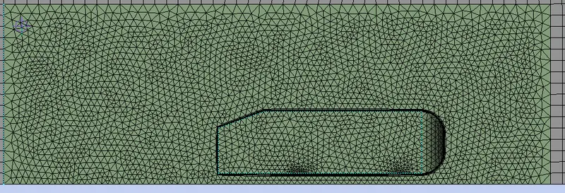
Mesh
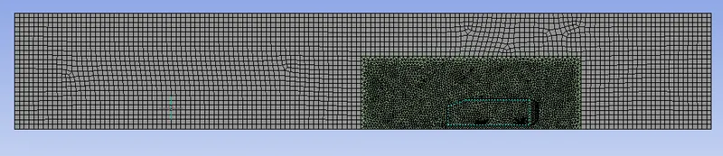
Outer domain element size = 55 mm
Body mesh element size = 27 mm
Drag Coefficient
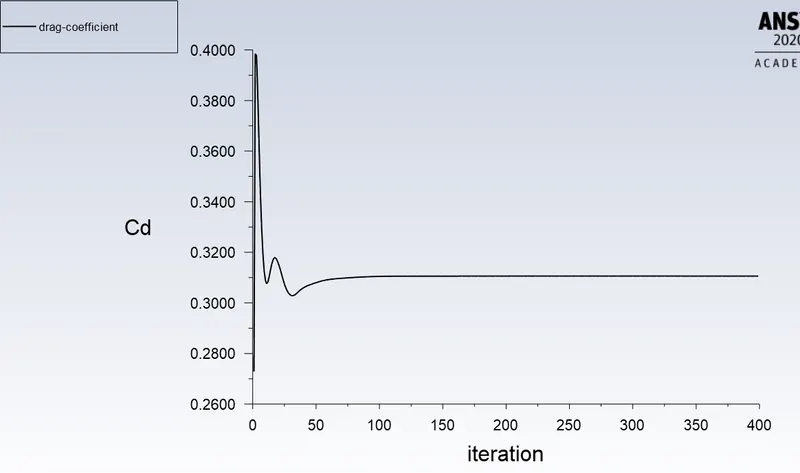
We can see that the graph is repeating the same pattern after some iteration so we get the converged value. The drag coefficient we get is 0.3142.
Pressure Contour
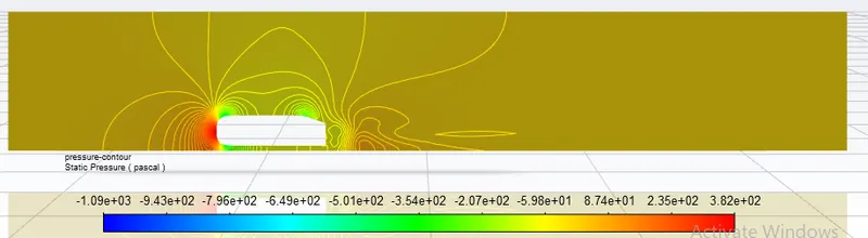
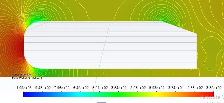
In the above figure, we can see that the pressure distribution in the entire domain. So we can see from the graph that at the inlet of Ahmed body pressure is higher. When we compare this to the first case we can see that we got the pressure to be in the same range and they look almost the same.
Velocity Contour
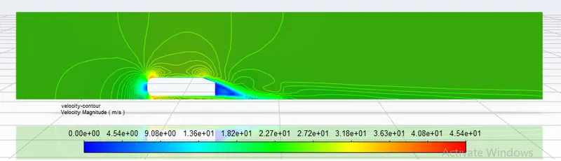
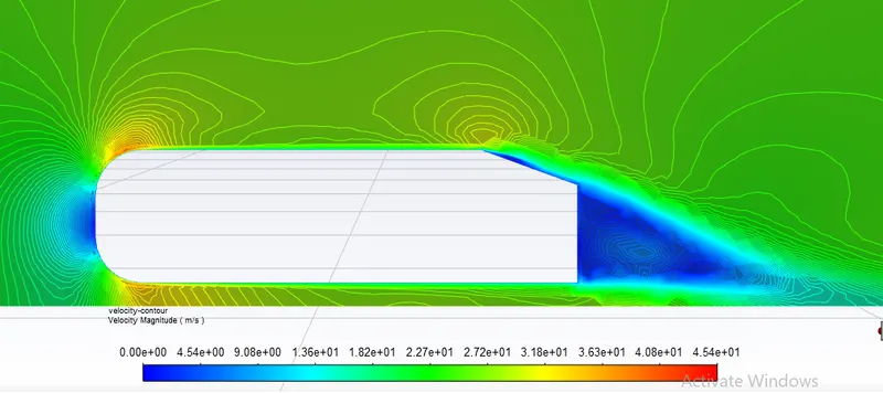
We can see from the contour that how is the velocity distribution in the domain. We are getting the velocity to be zero at the end of Ahmed's body that is the wake region. The range of the velocity is also the same as the previous case and they look almost the same.
Vector Plot
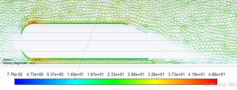
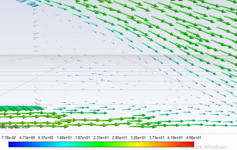
This is the vector plot in which we can see how the air is flowing around Ahmed's body. We can see that at the wake region air is in very small amount. same as the previous case.
Case-3
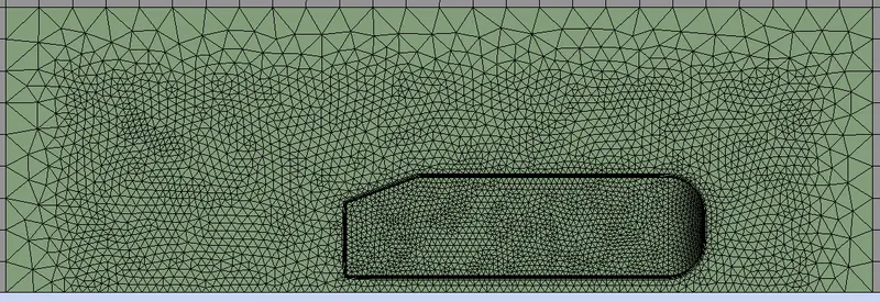
Mesh
Outer domain element size = 100 mm
Body mesh element size = 25 mm

Drag Coefficient
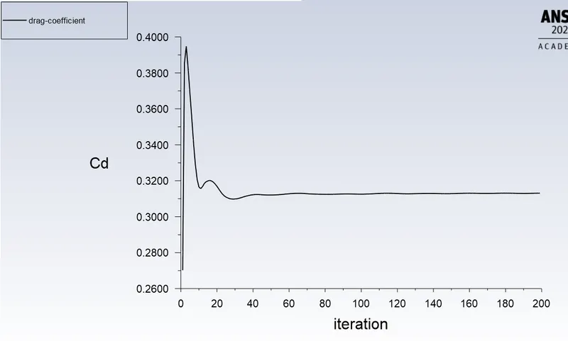
We can see that the graph is repeating the same pattern after some iteration so we get the converged value. The drag coefficient we get is 0.3131.
Pressure Contour
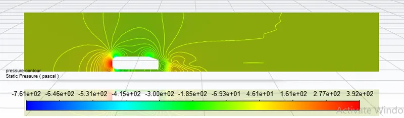
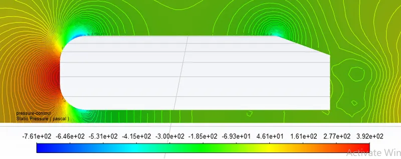
In the above figure, we can see that the pressure distribution in the entire domain. So we can see from the graph that at the inlet of Ahmed body pressure is higher. When we compare this to the first two cases we can see that the negative pressure decreases. But the region of the high and low pressure are the same.
Velocity Contour
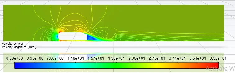
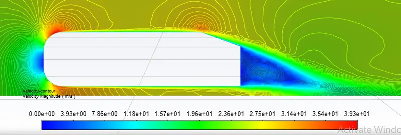
We can see from the contour that how is the velocity distribution in the domain. We are getting the velocity to be zero at the end of Ahmed's body that is the wake region. The maximum velocity value decreased in this case. But the region of the high and low pressure are the same.
Vector plot
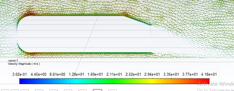
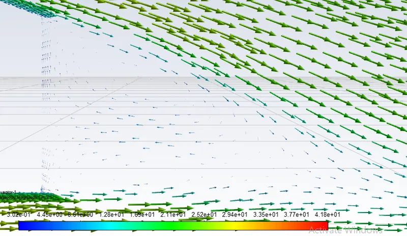
This is the vector plot in which we can see how the air is flowing around Ahmed's body. We can see that at the wake region air is in very small amount. same as the previous cases.
Comparision
| Case | Outer domain mesh size(mm) | Body mesh size (mm) | Number of elements | Drag coefficient | lift coefficient | Drag error % |
| case-1 | 55 | 30 | 342810 | 0.3179 | 0.2449 | 3.66 |
| case-2 | 55 | 27 | 437003 | 0.3142 | 0.2536 | 4.78 |
| case-3 | 100 | 25 | 480880 | 0.3131 | 0.2857 | 5.12 |
So from the table, we can see that the values are slightly different from each other. The error is around 5% so we can say that the simulation has passed the grid independence test. So our simulation is correct.
Conclusion
1. The high-pressure region occurs at the start of the body because of the decrease in the kinetic energy (based on Bernoulli's theorem). When the pressure is high, velocity decreases so the kinematic velocity also decreases.
2. Because of the sudden geometry change wake region is created. In the rear end of the body, there is some slant angle because of that there is sudden detachment of the body and air which's why the wake region created at the rear.
During the flow separation period, vortices are created downstream forming wake patterns.
3. When the body displaced, there is empty space creates. which is nothing but the wake region. Which creates a vacuum in that area. Because of the vacuum, there will be negative pressure.
4. If the wake region is bigger, eddies will be bigger and the drag force will be high. So the vehicle will consume more fuel. So to decrease the fuel consumption wake region should be small.
5. Point of the separation depends on the slant angle. The higher the slant angle, the point of separation will be early in the body. Lower the slant angle, the point of separation will be at the end of the body.
6. Size of the wake region depends upon the point of separation. If the point of separation is early in the body the wake region will be bigger. We want the wake region to be small. So the point of separation should be present as far as possible in the body.