1D Flame Speed Analysis

Aim: - To perform 1-D Flame Speed Analysis for Combustion of Methane (CH4) and Hydrogen (H2) Molecule.

Objective: -

1. To write a code in python to perform 1-D Flame analysis for Methane and Hydrogen by plotting Flame Speed and Temperature Plots along the width.
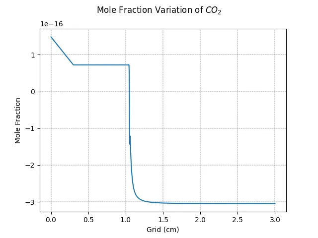
2. To plot the variation of concentration of CO2 for both analysis and its inference.

Theory: -

1-D Flame –

These are 1-D as certain Conditions i.e., no/negligible variation for properties in radial direction, are fulfilled. Hence the governing equations reduce to a system of ODEs in the axial coordinate.

The system or analysis consists of two regions unburnt/reactants and Burnt/products separated by a Flame Front.

Flame Speed –

The flow of species is conditioned to be laminar and is also denoted by laminar Flame speed (S_L). It is speed of diffusion of flame when ignite at a position and travelled to another end.

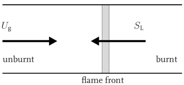
To make the problem easier, we assume the Flame front to be stationary and burnt gases propagates towards the front at relative speed equal to speed of Flame Front i.e. Flame speed. The unburnt gases are assumed to be moving far from the front.

Steady or Transient analysis?

Since Flame propagates and changes with time, thus a transient problem. But since transient analysis takes more Calculation capacity and time, we change the problem to steady state by fixing the point of reference i.e. flame front as shown above. Thus, the flame now becomes stationary for this problem and it is treated as steady state analysis.

For Methane (CH4) = gri30.xml

for Hydrogen (H2) = H2_mech.cti

same file should not be used for both reactions as both have different reaction mechanism hence different number of reactions are involved. the gri30 file can give result for H2 but it will be inaccurate as it is not calibrated for H2 but for CH4. H2_mech is calibrated according to mechanism for hydrogen combustion.

Code: -

• For methane Combustion

"""  
    1-D Flame speed or Methane 
"""

import cantera as ct 
import matplotlib.pyplot as plt


Tin = 300 
Pressure = ct.one_atm
reactant = 'CH4:0.45, O2:1, N2:3.76'

width = 0.03 

gas = ct.Solution('gri30.xml', 'gri30_mix')
gas.TPX = Tin , Pressure , reactant

f= ct.FreeFlame(gas, width = width)
f.set_refine_criteria(ratio=3, slope=0.07, curve=0.14)
f.solve(loglevel = 1)
Q_vol =abs(sum(f.standard_enthalpies_RT*f.net_production_rates)*ct.gas_constant*f.T)

print(f.grid, max(f.u), max(f.T))

plt.figure(1)
plt.subplot(3,1,1)
plt.suptitle('1-D Flame Speed Analysis For $CH_4$')
plt.plot(f.grid*100,f.T,'--')
plt.grid(axis ='both',color='k', ls = '-.', lw = 0.25)
plt.xlabel('Grid (cm)')
plt.ylabel('Temperature (K)')

plt.subplot(3,1,2)
plt.plot(f.grid*100,f.u,'--')
plt.grid(axis ='both',color='k', ls = '-.', lw = 0.25)
plt.xlabel('Grid (cm)')
plt.ylabel('Flame Velocity (m/s)')

plt.subplot(3,1,3)
plt.plot(f.grid*100,Q_vol,'--')
plt.grid(axis ='both',color='k', ls = '-.', lw = 0.25)
plt.xlabel('Grid (cm)')
plt.ylabel("Vol. Heat release")
plt.tight_layout()


plt.figure(2)
plt.plot(f.grid*100,f.X[gas.species_index('CO2')])
plt.grid(axis ='both',color='k', ls = '-.', lw = 0.25)
plt.xlabel('Grid (cm)')
plt.ylabel('Mole Fraction')
plt.suptitle('Mole Fraction Variation of $CO_2$')


plt.show()

Result: -

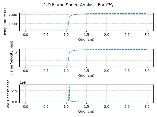
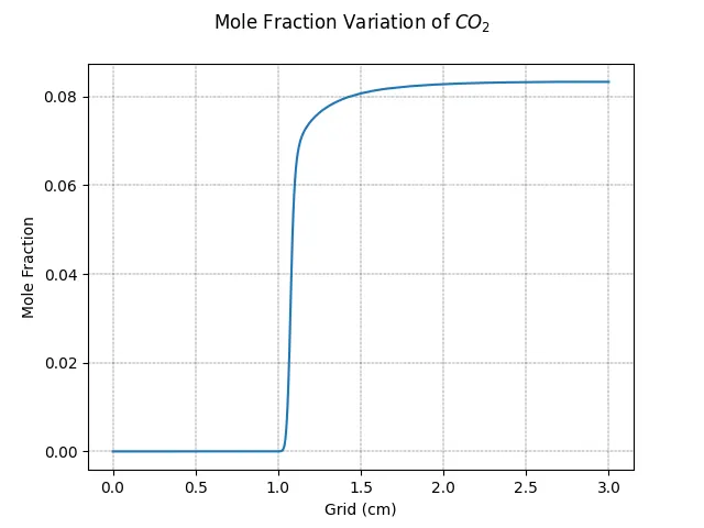
Max velocity reached = 2.427 m/sec

Max temperature = 2137.788 K

• For hydrogen combustion

"""  
    1-D Flame speed or H2 combustion
"""

import cantera as ct 
import matplotlib.pyplot as plt


Tin = 300 
Pressure = ct.one_atm
reactant = 'H2:0.45, O2:1'

width = 0.03 

gas = ct.Solution('H2_mech.cti')
gas.TPX = Tin , Pressure , reactant

f= ct.FreeFlame(gas, width = width)
f.set_refine_criteria(ratio=3, slope=0.07, curve=0.14)
f.solve(loglevel = 1)
Q_vol =abs(sum(f.standard_enthalpies_RT*f.net_production_rates)*ct.gas_constant*f.T)

print(f.grid, max(f.u), max(f.T))

plt.figure(1)
plt.subplot(3,1,1)
plt.suptitle('1-D Flame Speed Analysis For $H_2$')
plt.plot(f.grid*100,f.T,'--')
plt.grid(axis ='both',color='k', ls = '-.', lw = 0.25)
plt.xlabel('Grid (cm)')
plt.ylabel('Temperature (K)')

plt.subplot(3,1,2)
plt.plot(f.grid*100,f.u,'--')
plt.grid(axis ='both',color='k', ls = '-.', lw = 0.25)
plt.xlabel('Grid (cm)')
plt.ylabel('Flame Velocity (m/s)')

plt.subplot(3,1,3)
plt.plot(f.grid*100,Q_vol,'--')
plt.grid(axis ='both',color='k', ls = '-.', lw = 0.25)
plt.xlabel('Grid (cm)')
plt.ylabel("Vol. Heat release")
plt.tight_layout()

plt.figure(2)
plt.plot(f.grid*100,f.X[gas.species_index('CO2')])
plt.grid(axis ='both',color='k', ls = '-.', lw = 0.25)
plt.xlabel('Grid (cm)')
plt.ylabel('Mole Fraction')
plt.suptitle('Mole Fraction Variation of $CO_2$')


plt.show()

Result: -

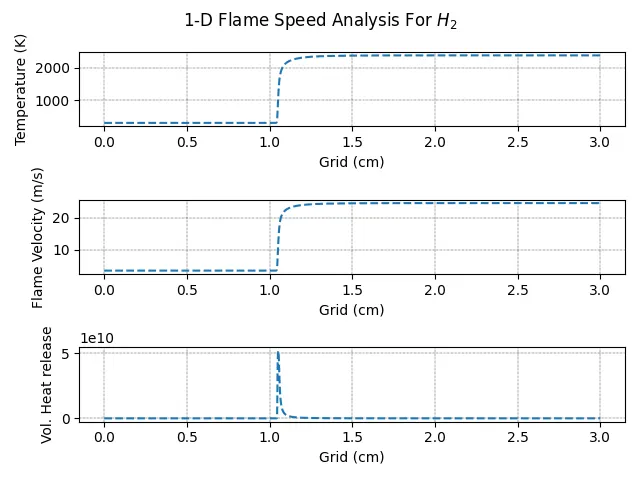
Max velocity reached = 24.489 m/sec

Max temperature = 2382.501 K

Conclusion: -

1. The flame speed for H2 combustion is higher than CH4 combustion for same mole o both the elements.
2. The mount of energy released for H2 is around 10 time of CH4 and since also have less molecular weight hence, Flame speed is higher for H2 combustion.
3. The one value to state for 1-D flame would be Flame speed as it has changed significantly than the temperture n higher the lme speed gives higher value of heat released.
4. The formation of CO2 in methane combustion is higher and since no presence of carbon in H2 hence negligible concerntration of CO2 in H2 combustion.
5. The width parameter does not significantly impact the result. It provides a region to solve for different Grid point to simulate a sence of propagation of flame. But since the flame front is assumed stationary hence width significance does not effect the solution.