50 CFD Engineer Interview Questions and Answers, With Worked Examples
The definitive CFD interview guide: 50 questions with model answers, from governing equations, discretisation, y+, turbulence models and mesh quality to ANSYS Fluent, OpenFOAM and STAR-CCM+, project and HR rounds, with worked y+, GCI and turbulence-inlet numbers and what candidates were asked at Praan, Hinduja Tech, Tech Mahindra and CADFEM.

In short
- CFD interviews in India test four things: fluid mechanics and the governing equations, numerics (discretisation, pressure-velocity coupling, convergence), meshing and turbulence modelling (y+ above all), and whether you really did the project on your CV.
- This guide has 50 questions with model answers, from first principles to ANSYS Fluent, OpenFOAM and STAR-CCM+, plus the project and HR questions that decide close calls.
- Three answers come with worked numbers drawn by code: the first-cell height for a target y+, a three-mesh grid convergence index, and turbulence inlet values.
- At the end is what candidates told us they were asked at Praan, Hinduja Tech, Tech Mahindra and CADFEM.
The questions that come up most in CFD engineer interviews are: what y+ is and how you chose it, which turbulence model you used and why, how you checked mesh quality and mesh independence, how SIMPLE and PISO differ, which boundary conditions you set, and how you know your solution converged. Interviewers then push into one project from your CV until they find the edge of what you understand.
Courses: compare all 20 Skill-Lync CFD courses, from 12-week courses in ANSYS Fluent, OpenFOAM, CONVERGE and ANSA meshing to the PG Program in CFD, with fees, duration, projects and placement data in one table.
Below are 50 questions grouped the way a technical round usually flows. Each answer is short enough to say out loud in about a minute. Where a number helps, it is worked out, so you can show the method rather than recite a definition.
How is a CFD engineer interview usually structured?
Most CFD hiring in India, whether at engineering-services companies, OEM R&D centres or simulation consultancies, runs in some version of these rounds:
- Fundamentals: fluid mechanics, heat transfer and the governing equations. Freshers get most of their questions here.
- CFD methods: discretisation, solvers, meshing, turbulence models, boundary conditions and convergence.
- Tool and project deep-dive: you explain a project and the interviewer asks why you made each setup choice. Some companies add a short hands-on test in Fluent, STAR-CCM+, OpenFOAM or a pre-processor such as ANSA.
- HR and fit: why CFD, why this company, relocation, notice period.
The deep-dive round is where most candidates lose marks. A rehearsed definition of y+ is not enough if you can't say what your y+ was, and why.
Fluid mechanics and governing equations (Q1 to Q9)
1. What is CFD, and what are the stages of a CFD analysis?
Computational fluid dynamics solves the equations of fluid flow and heat transfer numerically on a mesh, instead of analytically or in a wind tunnel. Every analysis has three stages:
- Pre-processing: clean the geometry, define the fluid domain, mesh it, and set physics and boundary conditions.
- Solving: iterate the discretised equations until they converge.
- Post-processing: extract forces, pressure drops and temperatures, check them, and compare with test data or a benchmark.
A strong answer adds that most of the engineering judgement, and most of the time, goes into pre-processing.
2. What are the governing equations of fluid flow?
There are three conservation laws:
- Mass (the continuity equation).
- Momentum (the Navier-Stokes equations, which are Newton's second law for a fluid element).
- Energy (the first law of thermodynamics).
For a compressible flow you also need an equation of state such as the ideal gas law. For an incompressible flow, continuity reduces to ∇·u = 0. The dependent variables are velocity, pressure and temperature (and density, if compressible). The independent variables are the three space coordinates and time.
3. Where does the non-linearity in the Navier-Stokes equations come from?
From the convective term, (u·∇)u: velocity multiplies its own gradient. That term causes turbulence and makes the equations hard to solve. It is also why a CFD solver must iterate: it linearises the equations around the current guess, solves, updates, and repeats. Variable properties (density or viscosity that depend on temperature) add more non-linearity.
4. When can a flow be treated as incompressible?
When density changes are small enough to ignore. For a gas, the usual rule of thumb is a Mach number below about 0.3. The isentropic relation ρ/ρ₀ = (1 + 0.2M²)−2.5 gives a density change of about 4.4% at M = 0.3, and less below it. Liquids are almost always treated as incompressible, except in problems such as water hammer. Natural convection is a special case: density varies with temperature, so you use the Boussinesq approximation or an incompressible-ideal-gas law, even though the flow is slow.
5. What is the Reynolds number? Work one out.
Re = ρUL/μ = UL/ν. It is the ratio of inertial to viscous forces and tells you whether a flow is laminar or turbulent. For pipe flow, Re below about 2,300 is laminar and above about 4,000 is turbulent, with a transitional range in between.
Worked example: air at 20 °C (μ = 18.13 × 10⁻⁶ Pa·s, ν = 15.06 × 10⁻⁶ m²/s, so ρ = 1.204 kg/m³) flowing at 30 m/s along a 4 m car gives Re = 30 × 4 / 15.06 × 10⁻⁶ ≈ 8.0 × 10⁶. That is fully turbulent, so a turbulence model is needed.
6. What is a boundary layer, and what causes flow separation?
Because of the no-slip condition, velocity at a wall is zero and rises to the free-stream value across a thin boundary layer, where viscosity matters. In a favourable pressure gradient (pressure falling downstream, as in a converging nozzle) the boundary layer stays attached. In an adverse pressure gradient (pressure rising, as on the rear of a car or the suction side of a stalled aerofoil) the slow fluid near the wall runs out of momentum, reverses and separates. Separation raises pressure drag and creates the wake. Predicting where it happens is the main job of the turbulence model and the near-wall mesh.
7. Explain the non-dimensional numbers you use in heat transfer.
- Prandtl number, Pr = ν/α: momentum diffusivity divided by thermal diffusivity. It sets the ratio of the velocity boundary layer to the thermal boundary layer: gases sit near 1, while water and oils are well above 1, so their thermal boundary layers are thinner than their velocity boundary layers.
- Nusselt number, Nu = hL/kfluid: convective heat transfer divided by pure conduction across the fluid.
- Biot number, Bi = hL/ksolid: resistance inside the solid divided by resistance at its surface. If Bi is well below 0.1, the solid is close to one uniform temperature (a lumped model works).
- Péclet number, Pe = Re × Pr: advection of heat divided by its diffusion.
- Grashof and Rayleigh numbers (Ra = Gr × Pr) measure how strong buoyancy is in natural convection.
Correlations usually take the form Nu = C Rem Prn.
8. What are static, dynamic and total pressure? What is gauge pressure in Fluent?
Static pressure is the thermodynamic pressure the fluid exerts. Dynamic pressure is ½ρV². Total (stagnation) pressure is their sum for incompressible flow, and it is the pressure you would measure if you brought the flow to rest without losses.
Gauge pressure is pressure measured relative to a reference. ANSYS Fluent solves for gauge pressure relative to a user-set operating pressure, and absolute pressure = operating pressure + gauge pressure. Fluent does this to avoid round-off error: small pressure differences are lost if you store them on top of 101,325 Pa. So when someone asks how Fluent knows whether a boundary value is gauge or absolute, the answer is that boundary pressures are always gauge, relative to the operating pressure you set.
9. What is the difference between an eddy, a vortex and vorticity? What is vortex shedding?
Vorticity (∇ × u) is a field quantity: it measures local rotation at a point. A vortex is a coherent region of fluid swirling around an axis. An eddy is the looser term for a swirling structure in turbulence, from the large energy-carrying eddies down to the smallest ones, where viscosity dissipates the energy as heat.
Vortex shedding is the alternating release of vortices from either side of a bluff body, such as a cylinder or a chimney. It causes oscillating lift, and it is the reason a "steady" cylinder case often won't converge: the physics is unsteady, so you need a transient run.
Discretisation, solvers and convergence (Q10 to Q19)
10. FVM, FEM and FDM: what is the difference, and why do most CFD codes use FVM?
- The finite difference method replaces derivatives with differences at grid points. It is simple, but it is awkward on complex geometry.
- The finite element method multiplies the equations by weighting functions and integrates them over elements (a weak, variational form). It dominates structural analysis.
- The finite volume method integrates the equations in conservation form over each control volume and balances fluxes through the faces.
Because the flux leaving one cell is exactly the flux entering its neighbour, FVM conserves mass, momentum and energy cell by cell, even on a coarse mesh. It also works on any cell shape. That is why Fluent, STAR-CCM+ and OpenFOAM are all finite volume codes.
11. Upwind or central differencing? What is numerical diffusion?
Convection schemes estimate face values from cell values. First-order upwind takes the value from the upstream cell. It is very robust, but it smears gradients as if extra viscosity had been added. That error is called numerical diffusion (or numerical viscosity), and it is worst when flow crosses the mesh at an angle. Second-order upwind and bounded central schemes are more accurate, but they can oscillate.
The usual practice is to start with first order for stability, switch to second order for the final answer, and never report results from a first-order run as final.
12. What is the Courant number, and how do you choose a time step? Work one out.
The Courant (CFL) number is C = UΔt/Δx: how many cells a fluid particle crosses in one time step. Explicit schemes are only stable for C ≤ 1 (lower for some schemes). Implicit solvers stay stable at larger C, but accuracy still needs the time step to resolve the physics you care about.
Worked example: for 30 m/s flow through 2 mm cells, C = 1 needs Δt = 0.002 / 30 ≈ 6.7 × 10⁻⁵ s. For vortex shedding, also check that each shedding period is covered by enough time steps (often 20 or more is a reasonable starting point). Then halve the step and confirm the result doesn't change.
13. Explain SIMPLE, SIMPLEC, PISO and the coupled solver.
In incompressible flow, pressure has no equation of its own; it is whatever value makes the velocity field satisfy continuity. Pressure-velocity coupling algorithms handle this:
- SIMPLE (Patankar and Spalding, 1972): guess the pressure, solve momentum, then solve a pressure-correction equation and correct the velocity and pressure. It needs under-relaxation and is the workhorse for steady flow.
- SIMPLEC (Van Doormaal and Raithby, 1984): a consistent approximation in the correction step that allows less under-relaxation on pressure. It often converges faster on simple flows, and it is not less accurate, since the converged answer is the same.
- PISO (Issa, 1986): one predictor plus two or more corrector steps within each time step. It was designed for transient flow with small time steps. OpenFOAM's PIMPLE combines PISO with SIMPLE-style outer loops, so it can take larger time steps.
- Coupled solvers solve momentum and pressure together in one matrix. They use more memory per iteration but need fewer iterations, and they are robust for difficult steady cases.
14. Pressure-based or density-based solver: when do you use each?
A pressure-based solver derives pressure from continuity through a correction equation. It is the default for incompressible and low-Mach flows, and it now handles a wide range of compressible flows too. A density-based solver solves continuity, momentum and energy together, with density as the primary variable. It is best for high-speed compressible flow with shocks, such as supersonic nozzles or re-entry. At very low Mach numbers it becomes stiff unless preconditioning is used.
Follow-up: implicit versus explicit: how does the answer differ in CFD and in FEA?
In CFD, an explicit scheme computes the new value from known old values. It is cheap per step but limited by the CFL condition. An implicit scheme solves a system of equations that couples the unknown new values, which allows bigger steps. In structural FEA the same words are used for crash (explicit, tiny time steps, LS-DYNA or Radioss) versus static or slow events (implicit). CAE interviews often ask both, so say which context you mean.
15. What is under-relaxation, and why is it needed?
Under-relaxation blends the new solution with the old one: φnew = φold + α(φcomputed − φold), with α below 1. It damps the swings that come from solving non-linear, coupled equations one at a time. Too low a value and convergence crawls. Too high and the residuals oscillate or diverge. Under-relaxation changes the path to the answer, not the converged answer.
16. How do you know a steady simulation has converged?
Never by residuals alone. Look for three things together:
- Scaled residuals have dropped several orders of magnitude and flattened out.
- The quantities you will report (drag, pressure drop, outlet temperature) are flat over hundreds of iterations.
- Mass and energy imbalances between inlets and outlets are a tiny fraction of the throughput.
If the residuals stall at a level while the monitored values oscillate, the flow may be physically unsteady, and a transient run is the honest fix.
17. What is the difference between boundary conditions and initial conditions?
Boundary conditions are values or fluxes held on the edges of the domain throughout the solution. Initial conditions are the starting field inside the domain. For a steady problem, a good initial field affects only how fast and how reliably you converge, not the answer. For a transient problem, the initial condition is part of the physics and must be realistic.
When you initialise in Fluent, the solver fills every cell with starting values. Standard initialisation copies constant values from a boundary or from user input. Hybrid initialisation builds a smoother, more physical starting field by solving simplified equations. That is why it often helps a difficult case start.
18. Which boundary conditions do you use, and which combinations are well posed?
- Inlets: velocity inlet, mass-flow inlet, or pressure (total-pressure) inlet.
- Outlets: pressure outlet (static pressure specified), or an outflow condition in some codes.
- Walls: no-slip, or slip or specified shear; stationary or moving; with a thermal condition (temperature, heat flux or convection).
- Symmetry and periodic boundaries to reduce domain size, and pressure far-field for external compressible aerodynamics.
A robust combination for internal flow is a velocity or mass-flow inlet with a pressure outlet. If you fix velocity at both ends, the problem becomes over-constrained.
A common follow-up asks what you could use instead of a velocity inlet for an Ahmed-body case. Answers include a pressure inlet with a known total pressure, or a symmetry or slip top boundary with a moving ground to match a rolling-road wind tunnel. Also place the outlet far enough downstream that the wake does not reach it, and confirm this by moving the outlet and checking that the result does not change.
19. What does "parametric study" mean in CFD?
Running the same validated setup while changing one or more inputs, such as inlet velocity, a fin pitch or a duct angle, to see how the outputs respond. The key is to change only what you mean to change: keep the meshing rules, models and convergence criteria identical, so differences between runs reflect the design, not the setup. Tools such as Fluent's design points or a Python script that drives the solver make this repeatable.
Meshing, y+ and mesh independence (Q20 to Q27)
20. How do you check mesh quality?
The main metrics:
- Skewness (how far a cell is from an ideal equilateral shape).
- Orthogonality (the angle between the line joining two cell centres and the normal of the face they share; Fluent reports it as orthogonal quality, from 0 = worst to 1 = best).
- Aspect ratio.
- Volume change between neighbouring cells.
- Negative or zero volumes, which are fatal.
Tolerances depend on the solver and version, so quote your tool's limits. For example, OpenFOAM's checkMesh flags non-orthogonality above 70°, skewness above 4 and aspect ratio above 1,000 by default. Pre-processors such as ANSA and HyperMesh add element checks like warpage, Jacobian and minimum angle. Long, thin prism cells in the boundary layer are fine as long as they are aligned with the flow; high aspect ratio there is intended, not an error.
21. Tetrahedral, hexahedral, polyhedral or prism cells: which and why?
- Hex cells are accurate and efficient when aligned with the flow, but hard to generate on complex geometry.
- Tet cells mesh anything automatically, but you need many more of them for the same accuracy, and they suffer more numerical diffusion.
- Polyhedral cells, built by merging tets, have many neighbours, so gradients are estimated better with fewer cells.
- Prism (inflation) layers capture the steep velocity and temperature gradients at walls.
Siemens' guide to Simcenter STAR-CCM+, for example, recommends the polyhedral or trimmed (hex-dominant) mesher for flow, with prism layers on walls. Tets are reserved mainly for solid and thermal FE meshes. If asked "tetra or hexa in ICEM CFD?", say hexa for a simple or flow-aligned geometry where blocking is practical, and tetra plus prisms when the geometry is too complex to block in the time available.
22. What is the difference between conformal and non-conformal meshes?
In a conformal mesh, neighbouring regions share nodes and faces exactly at their interface, so fluxes pass through without interpolation. A non-conformal mesh lets each region be meshed independently (for example a fine heat-sink mesh next to a coarse cabinet mesh in Icepak, or a rotating zone). The solver then interpolates fluxes across the interface. That is flexible, but it adds a small conservation and interpolation error, so keep interface cell sizes similar.
23. What is y+, and why does it matter?
y+ is the wall distance of the first cell centre, made non-dimensional with the friction velocity: y+ = y·uτ/ν, where uτ = √(τw/ρ). It tells you which layer of the boundary layer your first cell sits in, and that decides which wall treatment is valid:
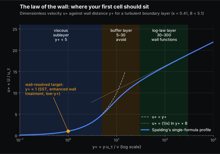
- Wall-resolved (k-ω SST, enhanced wall treatment in Fluent, low-y+ in STAR-CCM+): put the first cell centre at y+ of about 1. The Fluent user guide asks for at least 10 cells inside the viscosity-affected near-wall region.
- Wall functions (standard k-ε with standard wall functions): put the first cell centre in the log layer, roughly 30 < y+ < 300, preferably nearer 30.
- Avoid the buffer layer (about 5 to 30), where neither approach is accurate. Modern "y+-insensitive" or "all-y+" treatments blend the two so the result degrades gracefully, but they don't remove the need to know where you are.
24. How do you calculate the first-cell height for a target y+? Work it out.
Before meshing, estimate the wall shear from a flat-plate skin-friction correlation, then invert the definition of y+:
- Re = ρUL/μ
- Cf = [2 log₁₀(Re) − 0.65]−2.3 (Schlichting, valid for Re < 10⁹)
- τw = Cf · ½ρU²
- uτ = √(τw/ρ)
- y = y+ · μ / (ρuτ)
Worked for a 4 m car in air at 30 m/s (108 km/h):
- Re = 7.97 × 10⁶
- Cf = 0.00267
- τw = 1.45 Pa
- uτ = 1.096 m/s
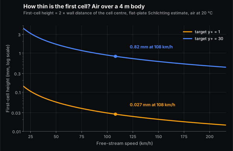
For y+ = 1, y = 1 × 18.13 × 10⁻⁶ / (1.204 × 1.096) = 0.0137 mm. For y+ = 30, y = 0.41 mm.
Here is the catch most candidates miss: y is the distance to the cell centre, and the solver reports y+ at the centroid. In a cell-centred finite volume code, the first cell height is therefore about 2y: 0.027 mm for y+ = 1, and 0.82 mm for y+ = 30. The estimate is a starting point. After the first run, plot the actual y+ contour on the walls and adjust, because local wall shear is much higher near stagnation points and much lower near separation.
25. What is a prism (inflation) layer, and how do you size it?
Thin, stacked prism or hex cells grown off walls, so that the cells are fine in the wall-normal direction (to resolve the gradient) but not in the wall-parallel direction (to save cells). Set three numbers:
- The first-layer height, from the y+ estimate above.
- The growth ratio between layers.
- The number of layers, or the total thickness, so the stack covers the boundary layer and the last layer's size blends into the core mesh.
If the last prism layer is much thinner than its neighbouring core cell, that sudden jump hurts accuracy and convergence. In STAR-CCM+, the prism layer thickness depends on the wall y+ treatment you select.
26. What is a mesh independence study? Show a grid convergence index calculation.
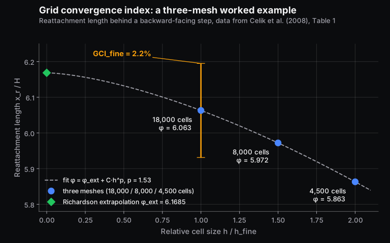
You solve the same case on at least three systematically refined meshes and check that the quantity you care about stops changing. The grid convergence index (GCI) method, published as the ASME Journal of Fluids Engineering procedure by Celik and co-authors in 2008, turns this into a reported uncertainty:
- Compute a representative cell size h for each mesh, and keep the refinement ratio r = hcoarse/hfine above 1.3.
- Find the apparent order of accuracy p from the three solutions φ₁ (fine), φ₂ and φ₃.
- Extrapolate: φext = (rpφ₁ − φ₂)/(rp − 1).
- Report GCIfine = 1.25 ea/(rp − 1), where ea = |(φ₁ − φ₂)/φ₁|.
Using the paper's own example, the reattachment length behind a backward-facing step on 18,000, 8,000 and 4,500 cells was 6.063, 5.972 and 5.863. In 2D, h ∝ N−1/2, so r₂₁ = 1.5 and r₃₂ = 1.333. Recomputing it gives:
- apparent order p = 1.53
- φext = 6.1685
- ea = 1.5%
- GCIfine = 2.2%, matching the paper
So you would report the fine-mesh reattachment length as 6.063 with a numerical uncertainty of about 2.2%. That covers discretisation only, not turbulence-model error.
27. Meshing-role questions: surface mesh, volume mesh and ANSA checks
Interviews for CFD pre-processing roles (often using ANSA or HyperMesh) go deep into meshing:
- Why build a surface mesh first? The volume mesh grows from it, so surface quality (size transitions, captured features, no free edges or overlaps) limits everything after.
- Why prisms at the wall? To resolve the boundary layer cheaply (see Q25).
- What are warpage and Jacobian? Warpage measures how far a quad's nodes are from lying in one plane. Jacobian measures how distorted an element is from its ideal shape; 1 is ideal, and values near zero or negative mean a degenerate element.
- What does morphing do? It changes the shape of an existing mesh (for a design change or optimisation) without remeshing from scratch.
- What is an ideal triangle? An equilateral one, with 60° angles and zero skewness.
- What do you check before delivery? Free and duplicate edges, intersections and penetrations, quality criteria against the customer's limits, correct property and material IDs, and the part naming convention.
Be ready to answer quads-versus-trias questions honestly. Warpage is defined for quads, so it shows up there; trias are always planar but are stiffer and less accurate in FE shell meshes.
Turbulence modelling (Q28 to Q33)
28. Why do we need turbulence models? Compare DNS, LES and RANS.
- DNS resolves every eddy down to the dissipative scale. Its cost grows steeply with Reynolds number, so it is a research tool.
- LES resolves the large, energy-carrying eddies and models only the small ones. It is accurate for separated and unsteady flow, but it needs fine meshes and long transient runs.
- RANS splits every variable into a mean and a fluctuation (Reynolds decomposition) and solves only for the mean. Averaging creates new unknowns, the Reynolds stresses, which a turbulence model must supply. This is the closure problem.
RANS is the industry workhorse because it runs as a steady simulation on a modest mesh. Hybrid RANS-LES methods (DES, DDES) use RANS near walls and LES in separated regions.
29. What are k, ε and ω? How do k-ε, k-ω and SST differ?
k is the turbulent kinetic energy (energy in the velocity fluctuations), ε is its rate of dissipation, and ω is the specific dissipation rate (roughly ε/k, a turbulence frequency). In the main two-equation models:
- Standard k-ε: robust and cheap for free-shear and internal flows. It needs wall functions and tends to over-predict turbulence and delay separation in adverse pressure gradients.
- k-ω (Wilcox): integrates down to the wall and handles adverse pressure gradients better, but it is sensitive to the free-stream value of ω.
- k-ω SST (Menter, 1994): uses k-ω near the wall and k-ε away from it through a blending function, and limits the turbulent shear stress so separation is predicted more realistically. It is the default first choice for external aerodynamics and most wall-bounded flows.
30. Which turbulence model would you use for external aerodynamics, and why not k-ε?
Usually k-ω SST with a wall-resolved mesh (y+ about 1), because drag on a car or aerofoil depends on where the boundary layer separates. Standard k-ε with wall functions tends to keep the flow attached too long. For aerospace attached flows, the one-equation Spalart-Allmaras model is also widely used and cheap. If the wake is large and unsteady (a bluff truck, or a cylinder at high Re), mention that RANS has limits there and that DES or LES may be justified. Then mention cost, because interviewers like candidates who weigh accuracy against compute.
31. Wall functions or a resolved boundary layer?
Wall functions bridge the near-wall region with the log-law formula, so the first cell can be much thicker (y+ 30 to 300). That saves cells on big industrial models such as HVAC ducts, engine bays and buildings. A resolved boundary layer (y+ about 1) is needed when wall shear, heat transfer or separation are the answer you are being paid for: drag, pressure drop through a separating diffuser, or a heat transfer coefficient on a turbine blade. The STAR-CCM+ all-y+ and Fluent y+-insensitive treatments blend the two, so a mixed-y+ mesh still gives sensible answers.
32. How do you set turbulence at an inlet? Work it out.
Usually as an intensity I and a length scale ℓ (or a viscosity ratio). The Fluent user guide gives the conversions:
- I ≈ 0.16 ReD−1/8 for fully developed duct flow
- ℓ ≈ 0.07 Dh
- k = 1.5(UI)²
- ε = Cμ3/4k3/2/ℓ
- ω = k1/2/(Cμ1/4ℓ), with Cμ = 0.09
The same guide calls 1% or less low intensity and above 10% high.
Worked: air at 10 m/s in a 0.1 m duct gives Re = 66,400, then:
- I = 4.0%
- ℓ = 7 mm
- k = 0.239 m²/s²
- ε = 2.75 m²/s³
- ω = 128 s⁻¹
33. What is the Boussinesq eddy-viscosity hypothesis, and where does it fail?
It assumes the Reynolds stresses are proportional to the mean strain rate through a scalar turbulent viscosity μt, just as molecular stress is in a Newtonian fluid. Two-equation models (k-ε, k-ω, SST) all use it. It fails where turbulence is strongly anisotropic: secondary flows in square ducts, strong swirl, streamline curvature. Reynolds-stress models solve a transport equation for each stress component instead, at higher cost and with weaker robustness.
Heat transfer, multiphase and moving parts (Q34 to Q38)
34. What is conjugate heat transfer (CHT)? Explain it with an electronics example.
CHT solves conduction in solids and convection in the fluid together, with temperature and heat flux continuous at the interface, rather than guessing a heat transfer coefficient on the wall. A classic interview version: a graphics card in a box.
- Heat generated in the GPU die conducts through the package and heat sink.
- It convects into air driven by the fans.
- Some leaves by radiation.
Numerically, you mesh the solids and the air, assign a volumetric heat source to the die, model the fans (as a fan boundary condition, a momentum source or an MRF zone), and couple the solid and fluid regions at their interfaces. Be ready to state the box size and the boundary conditions of your own project; "project-specific" questions like this test whether you did the work yourself.
35. What is the heat transfer coefficient, and how does CFD calculate it?
Newton's law of cooling defines it: q = h(Twall − Tref). Analytically you get h from a Nusselt correlation, h = Nu·k/L. In CFD the solver computes the wall heat flux directly, and h is derived from it. That means h depends on the reference temperature you choose (inlet, bulk or a fixed value), and on near-wall mesh resolution, because heat flux is a wall gradient just like shear. Two engineers can report different h for the same simulation if they use different references, so always state yours.
36. How do you simulate natural convection?
Switch on gravity, model the density change with temperature (the Boussinesq approximation for small temperature differences, or an incompressible-ideal-gas law for larger ones), and check the Rayleigh number to decide between a laminar and a turbulent model. Set the operating density sensibly so the hydrostatic pressure doesn't swamp the buoyancy-driven differences, and resolve the thin thermal boundary layers on hot walls. These cases converge slowly and are sometimes genuinely unsteady.
37. VOF, Eulerian or DPM: which multiphase model and when?
- VOF tracks a sharp interface between immiscible fluids: tank sloshing, free-surface flow, filling.
- Eulerian-Eulerian (multi-fluid) treats each phase as an interpenetrating continuum with its own velocity: fluidised beds, bubble columns, any case where the dispersed phase is dense.
- DPM (Euler-Lagrange) tracks individual particles or droplets through a continuous phase: sprays, dust, fuel injection, particles in an air purifier. The Fluent user guide states that DPM assumes the dispersed phase is dilute, usually below 10 to 12% by volume.
So the honest answer to "which is more accurate?" is that it depends on the volume fraction and on whether you need individual particle histories. Lagrangian tracking is efficient for dilute flows but becomes expensive and invalid as loading rises.
A related question is the slip ratio in gas-liquid flow: the ratio of gas velocity to liquid velocity. Homogeneous models assume it equals 1; separated-flow models allow the phases to move at different speeds.
38. MRF or sliding mesh for rotating machinery?
The moving reference frame (MRF, or frozen rotor) approach solves the rotating zone in a rotating frame on a stationary mesh. It is steady and cheap, and good for performance curves of fans and pumps. A sliding mesh physically rotates the zone each time step across a non-conformal interface. It is transient and expensive, but it captures blade-passing pulsations and rotor-stator interaction. A sensible workflow is to converge MRF first and use it to initialise a sliding-mesh run.
Tool-specific questions: ANSYS Fluent, OpenFOAM, STAR-CCM+ (Q39 to Q45)
39. (Fluent) What do you check before trusting a Fluent result?
Run through this list:
- Mesh check and quality report clean, with no negative volumes.
- Units and scale correct (a CAD model imported in millimetres as metres is a classic mistake).
- Material properties at the right temperature.
- Operating pressure and gravity set deliberately.
- Boundary condition types and directions correct.
- Second-order discretisation for the final run.
- Monitors of the reported quantities flat.
- Mass and heat flux reports balanced.
- Wall y+ checked against the model's requirement.
Saying this as a checklist shows you have run real cases.
40. (Fluent) A case diverges with floating-point errors. What do you do?
Work from the cause, not from the symptom:
- Look at where the residual spike lives (mark high-residual cells, or check the worst-quality cells).
- Fix bad cells in that region.
- Check boundary conditions for reverse flow at outlets.
- Restart from a converged first-order solution.
- Lower under-relaxation or the Courant number temporarily.
- Use hybrid initialisation, or ramp up inlet velocity or heat load in steps.
Then explain how you would confirm the fix did not just hide a real physical instability.
41. (OpenFOAM) Describe an OpenFOAM case structure and its meshing tools.
A case has three folders:
0/holds the initial and boundary conditions for each field (U, p, k, omega, nut).constant/holds the mesh (polyMesh) and physical properties (transport and turbulence models).system/holds the run controls:controlDict,fvSchemes(discretisation) andfvSolution(linear solvers, SIMPLE or PIMPLE settings, relaxation).
blockMesh builds structured hex blocks, often the background mesh. snappyHexMesh then works in three switchable stages: castellatedMesh (refine and remove cells outside the geometry), snap (move boundary points onto the surface) and addLayers (insert near-wall layers). Run checkMesh afterwards.
42. (OpenFOAM) simpleFoam, pimpleFoam or icoFoam?
icoFoam: transient, incompressible, laminar, PISO. It is a teaching solver.simpleFoam: steady, incompressible, turbulent (RANS), SIMPLE.pimpleFoam: transient, incompressible, turbulent, PIMPLE, so it can run at larger Courant numbers with outer correctors.
Compressible, buoyant and multiphase cases use their own solver families. In recent OpenFOAM versions several of these have been merged into modular solvers, so mention the version you used.
43. (STAR-CCM+) How do you mesh and set up a typical case in STAR-CCM+?
The usual path is:
- Import and repair the surface, then assign parts to regions and set boundary types before meshing (so prism layers grow on walls).
- Run an automated mesh operation with a surface remesher, a core volume mesher (polyhedral for most internal flows, trimmed hex for external aerodynamics) and the prism layer mesher.
- Choose physics models in a continuum: segregated or coupled flow, steady or implicit unsteady, a turbulence model with a wall treatment (low-y+, high-y+ or all-y+).
- Drive the run with reports, monitors and stopping criteria. Automate repetitive work with Java macros.
44. Which CFD software do you prefer, and why?
There is no right tool. There is a right reason. A good answer names a tool you have actually used and ties the preference to a task. For example: "Fluent for its range of physics and fast setup on industrial models; OpenFOAM when I need to see or change the discretisation, or run many cores with no licence limit; STAR-CCM+ for its automated polyhedral and prism meshing on dirty CAD." Then add one honest limitation of your preferred tool. Avoid claiming deep expertise in a tool you have only seen in a tutorial; the next question will expose it.
45. Have you automated any CFD work?
Interviewers increasingly ask this because most production CFD is repetitive. Examples worth mentioning, if you have done them:
- A Fluent journal or Python (PyFluent) script that loops over design points.
- A STAR-CCM+ Java macro that exports reports.
- Bash or Python scripts that run OpenFOAM cases and post-process with ParaView.
- ANSA or HyperMesh scripts (Python, or Tcl/Tk) for batch meshing.
Mention what it saved, in hours or number of cases.
Project and behavioural questions (Q46 to Q50)
46. Walk me through a CFD project you did.
Use a fixed structure and real numbers:
- Objective: what decision the simulation supported.
- Domain and boundary conditions.
- Mesh: cell count, type, first-layer height and achieved y+.
- Models: turbulence model, other physics, and why.
- Convergence evidence.
- Mesh independence: two or three meshes and how much the result changed.
- Validation against data.
- What you would do differently.
For an Ahmed-body project, for instance, quote the drag coefficient you got, the experimental value you compared against and the percentage difference. Then explain the gap (turbulence model, wake resolution, the slant-angle regime). An answer with numbers and a known limitation beats a polished answer without them.
47. How do you validate your CFD results?
Separate verification (did I solve the equations correctly: mesh independence, time-step independence, iterative convergence, a GCI estimate) from validation (did I solve the right equations: comparison with experiment, a published benchmark, or a hand calculation such as a pipe pressure drop from the Darcy-Weisbach equation). If you had no test data, say so and explain which sanity checks you used instead: mass balance, an order-of-magnitude drag estimate, comparison with a correlation.
48. How would you design and optimise an air purifier using CFD?
This question has come up at clean-air hardware companies. A good answer:
- Define what "better" means: clean-air delivery rate, pressure drop across the filter, noise, uniform flow through the filter face.
- Model the fan (MRF or a fan curve), the filter as a porous zone with resistance coefficients fitted to supplier data, and the room or test chamber.
- Track particles with DPM, which is valid because the loading is dilute.
- Vary inlet grille, filter placement and outlet louvre angle in a parametric study.
- Validate airflow against an anemometer measurement before trusting the particle results.
49. Why should we hire you for a CFD role?
Tie three things together: a CFD skill they need (from the job description), evidence you have it (a project with numbers), and how you work (you check your own results, you document setups, you automate repetitive work). Keep it under a minute and specific to the company: an automotive services firm cares about turnaround and process, a startup cares about range and ownership.
50. Tell me about yourself, and why CFD?
Give a 60-second version: degree and the subject that got you interested, the one or two CFD projects you are proudest of (with one number each), any training or certification, and what you want to work on next. "Why CFD" lands best when it is concrete: the first time a simulation predicted something you then saw in a test, or a design you improved because of a contour plot.
What did candidates say they were asked at specific companies?
Between September and November 2024, Skill-Lync published a series of "Engineer's Interview Blueprint" posts. Each was built from questions that learners reported after interviews for CFD and CAE roles, and those posts are now merged into this guide. Treat this as candidate-reported, not as an official question bank from the companies. It reflects particular interviews for particular roles.
- Praan (CFD engineer, clean-air hardware): DPM in Fluent, multiphase modelling, Euler-Euler versus Euler-Lagrange, CHT, time-step selection from the Courant number, SIMPLE versus PISO and SIMPLE versus SIMPLEC versus Coupled, mesh-quality checks, validation, natural convection, what happens when you initialise in ANSYS, automation and programming languages, and designing and optimising an air purifier.
- Hinduja Tech (CFD engineer): a list that overlapped heavily with Praan's (DPM, multiphase, CHT, time step, SIMPLE and PISO, validation, mesh quality, the air-purifier design question), plus the candidate's OpenFOAM project, meshing in OpenFOAM (blockMesh and snappyHexMesh) and the final-year project.
- Tech Mahindra (CFD engineer, automotive): mostly general engineering rather than CFD: petrol versus diesel engines, 2WD versus 4WD, EV and HEV basics, GD&T basics and dimensioning symbols, centre of gravity and degrees of freedom. Engineering-services roles often screen breadth first, so revise core mechanical and automotive basics too.
- CADFEM (CAE and simulation roles): FEA rather than CFD: implicit versus explicit, LS-DYNA material cards such as MAT 24 (piecewise linear plasticity), engineering versus true stress, quasi-static analysis, mass scaling, ANSA morphing, modal analysis, S-N curves and buckling.
- CFD meshing roles (company not named): ANSA versus HyperMesh, surface versus volume meshing, prism layers, skewness, warpage, Jacobian and aspect ratio, meshing sheet-metal versus plastic parts, lapping and morphing, and pre-delivery checks.
- General CFD rounds also included: Bernoulli's equation and its assumptions, kinematic viscosity and units, the continuity equation, gauge versus absolute pressure, eddy versus vortex versus vorticity, gas turbine cycles and why compressors need many stages while a turbine stage can take a large pressure drop (an adverse versus favourable pressure gradient question in disguise), pump cavitation, and solar thermal applications for candidates with that project on their CV.
The pattern is clear: the CFD core (y+, turbulence models, pressure-velocity coupling, mesh quality, CHT, multiphase) is asked everywhere, and the rest follows the company's domain and the projects on your CV.
How should you prepare in the two weeks before a CFD interview?
- Re-run one project end to end and write down every number: domain size, cell count, first-layer height, achieved y+, model, convergence criteria, result, validation gap.
- Practise the worked calculations in this guide by hand: Reynolds number, first-cell height, Courant time step, turbulence inlet values. Interviewers love "work it out on the whiteboard".
- Do a quick mesh independence study on a small case so you can talk about GCI from experience.
- Revise fundamentals in fluid mechanics and heat transfer: Bernoulli, boundary layers, non-dimensional numbers, the modes of heat transfer.
- Read the job description and prepare one example per tool or physics it lists.
If you want structured practice, Skill-Lync's Post Graduate Program in CFD covers solver development through to ANSYS Fluent and CONVERGE. There are also shorter courses: GUI-based CFD with ANSYS Fluent, Advanced CFD with OpenFOAM and CFD meshing with ANSA. For background reading, see what CFD is and how it works and boundary layers and near-wall regions in CFD.
Frequently asked questions
What are the most important CFD interview topics for freshers?
Governing equations and what each term means, Reynolds number and boundary layers, y+ and wall treatment, k-ε versus k-ω SST, SIMPLE versus PISO, mesh quality and mesh independence, boundary conditions, and one project you can explain with real numbers. Freshers are judged more on fundamentals and honesty about their project than on tool tricks.
What y+ value should I use?
About 1 for wall-resolved models (k-ω SST, enhanced wall treatment, low-y+) when drag, separation or heat transfer matter. Between about 30 and 300 for wall functions on large industrial models. Avoid roughly 5 to 30. Estimate the first-cell height before meshing (Q24), then check the y+ contour after the first run.
Is OpenFOAM or ANSYS Fluent better for getting a CFD job in India?
Many industrial jobs list ANSYS Fluent or STAR-CCM+ because companies already hold licences, while OpenFOAM experience signals that you understand the numerics and can work without a GUI. Learn one commercial tool well and know enough OpenFOAM to explain a case structure. Read each job description for the tool it names.
How many questions are asked in a CFD technical interview?
It varies widely by company and round. In the candidate reports we collected, a technical round covered roughly 8 to 20 questions, with the project discussion taking a large share of the time. Prepare depth on a few topics over shallow coverage of many.
Do CFD interviews include coding questions?
Sometimes. Expect questions on scripting and automation (Python, MATLAB, journals or macros) more than algorithm puzzles. Solver-development roles may ask you to discretise a 1D convection-diffusion equation or explain a stability limit.
Sources and further reading
- Celik, I. B., Ghia, U., Roache, P. J. and Freitas, C. J., Procedure for Estimation and Reporting of Uncertainty Due to Discretization in CFD Applications, ASME Journal of Fluids Engineering 130(7), 2008 (GCI procedure and Table 1 data)
- CFD Online Wiki, Y plus wall distance estimation, Law of the wall and Skin friction coefficient (accessed 14 Nov 2026)
- ANSYS FLUENT 12.0 User's Guide (public mirror, ENEA): 12.3.1 Near-wall mesh guidelines; 7.3.2 Turbulence boundary conditions; 8.14.2 Operating, gauge and absolute pressure; 23.1.2 DPM limitations
- OpenFOAM Foundation, primitiveMeshCheck.C (OpenFOAM-10 source: checkMesh default thresholds)
- CFD Direct, OpenFOAM User Guide: snappyHexMesh and case file structure
- Siemens Digital Industries Software, A new user's guide to Simcenter STAR-CCM+ simulation (Part 3/5): Meshing
- Menter, F. R., Two-equation eddy-viscosity turbulence models for engineering applications, AIAA Journal 32(8), 1994
- Spalding, D. B., A single formula for the "law of the wall", Journal of Applied Mechanics 28(3), 1961
- Patankar, S. V. and Spalding, D. B., A calculation procedure for heat, mass and momentum transfer in three-dimensional parabolic flows, International Journal of Heat and Mass Transfer 15, 1972 (SIMPLE)
- Van Doormaal, J. P. and Raithby, G. D., Enhancements of the SIMPLE method for predicting incompressible fluid flows, Numerical Heat Transfer 7, 1984 (SIMPLEC)
- Issa, R. I., Solution of the implicitly discretised fluid flow equations by operator-splitting, Journal of Computational Physics 62, 1986 (PISO)
- Engineering ToolBox, Air: dynamic and kinematic viscosity and Reynolds number (accessed 14 Nov 2026)
- NASA Glenn Research Center, Isentropic flow relations
- Skill-Lync Engineer's Interview Blueprint series (Sep to Nov 2024), candidate-reported questions from Praan, Hinduja Tech, Tech Mahindra and CADFEM interviews, merged into this page