Write code to fit a linear and cubic polynomial for the Cp data in MATLAB.

Write code to fit a linear and cubic polynomial for the Cp data in MATLAB.

Introduction:-

Polynomials are one of the significant conepts of mathematics and so are the types of polynomials that are determined by the degree of polynomials which further determines the maximum number of solutions a function could have and the number of times a function will cross the x-axis when graphed.

Objective:-

1. Write code to fit a linear and cubic polynomial for the Cp data.
2. Plot the linear and cubic fit curves along with the raw data points.
3. Write a code to show splitwise method.

Theory:-

The degree of polynomials is the highest exponential power in the polynomial equation. Only variables are considered to check for the degree of any polynomials, coefficient are to be ingnored. For an nth degree polynomials function with real coefficients and the variables is represented as x, having the highest power n, where n takes whole number values.

1. Linear polynomials:- A linear polynomial is a polynomial of degree one.

Example:- y = ax+b

2. Quadratic polynomials:- A quadratic polynomial is a polynomial of degree two.

Example:- y = ax^2+bx+c

3. Cubic polynomials:- A cubic polynomials is a polynomial of degree three.

Example:- y = ax^3+bx^2+cx+d

• parameters used to measure the fitness characteristics for both the curves:-

MSE, SSE, and R-square are used to measure fitness of the curve.

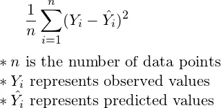
1. MSE (Mean Squared Error):- It is measures the average of the squares of the errors that is the average squared between the estimated values and the actual values. For the entire set of data. As suggested by its name, we take the average, or the mean, of the individual squared error terms in order to calculate MSE.

   Putting this all together, we have the general formula for calculating MSE:

   

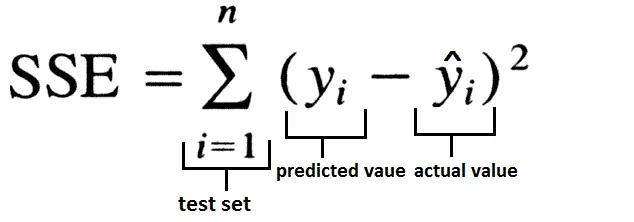
2. SSE (Sum of squared error):- It is measures the total deviation of the response values from the fit to the response values it is called as sum of squared error.

We have the general formula for calculating MSE:

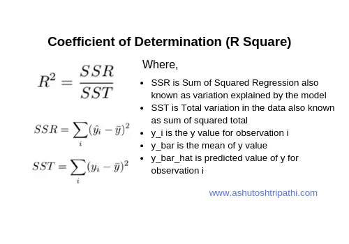
3. R-Square:- It is a statistical measure that represents the proportion of the variance for a dependent variable that's explained by an independent variable or variables in a regression model. It also known as coefficient of determination. R-squared values range from 0 to 1 and are commonly stated as percentages from 0% to 100%. In analysis R-squared value 1 is define perfect fit.

We have the general formula for calculating R-square:

Explanation of program:- Start the program using clear all, close all, clc. then loading the given data in matlab then seprate the column in given data as temperature and specific heat. then use polyfit command in coeff1 variable it computes a least-squares polynomial for a given set of data. It generates the coefficients of the polynomial, which can be used to model a curve to fit the data. and then use polyval command for evaluating a polynomial in a matrix sense using this command get actual linear fit curve of specific heat. then give plot command to graph a curve in actual and predicted linear fit curve of specific heat and give labeling and legend. and the same process again in quadratic polynomial and cubic polynomial but only change degree of polynomial. Then calculate R-square for all polynomials.

program:-

clear all
close all
clc

%load data file
dharmesh = load('data');
temperature = dharmesh(:,1);
cp = dharmesh(:,2);

%solve curve fit linear polynomial
%y = ax+b
coeff1 = polyfit(temperature,cp,1);
pred_cp1 = polyval(coeff1,temperature);

%solve curve fit quadratic polynomial
%y = ax^2+bx+c
coeff2 = polyfit(temperature,cp,2);
pred_cp2 = polyval(coeff2,temperature);

%solve curve fit cubic polynomial
%y = ax^3+bx^2+cx+d
coeff3 = polyfit(temperature,cp,3);
pred_cp3 = polyval(coeff3,temperature);

%plotting curve fit linear polynomial
figure(1)
plot(temperature,cp)
hold on
plot(temperature,pred_cp1)
xlabel('Temperature')
ylabel('Specific Heat')
title('Curve Fit Linear')
legend('actual cp','predicted cp')

%plotting curve fit quadratic polynomial
figure(2)
plot(temperature,cp)
hold on
plot(temperature,pred_cp2)
xlabel('Temperature')
ylabel('Specific Heat')
title('Curve Fit Quadratic')
legend('actual cp','predicted cp')

%plotting curve fit cubic polynomial
figure(3)
plot(temperature,cp)
hold on
plot(temperature,pred_cp3)
xlabel('Temperature')
ylabel('Specific Heat')
title('Curve Fit Cubic')
legend('actual cp','predicted cp')

%calculations
s = sum(cp);
mean = s/length(cp);

%for linear polynomial
for i = 1:length(cp);
    SSE1 = (cp(i)-pred_cp1(i))^2;
    SSR1 = (pred_cp1(i)-mean)^2;
end
    SST1 = SSR1+SSE1;
    R_square1 = SSR1/SST1;
    
    %for quadratic polynomial
for j = 1:length(cp);
    SSE2 = (cp(j)-pred_cp2(j))^2;
    SSR2 = (pred_cp2(j)-mean)^2;
end
    SST2 = SSR2+SSE2;
    R_square2 = SSR2/SST2;
    
    %for cubic polynomial
for k = 1:length(cp);
    SSE3 = (cp(k)-pred_cp3(k))^2;
    SSR3 = (pred_cp3(k)-mean)^2;
end
    SST3 = SSR3+SSE3;
    R_square3 = SSR3/SST3;

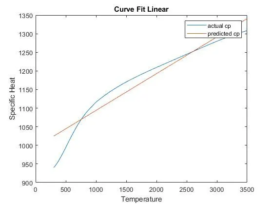
Plot1:- Linear polynomial curve fit

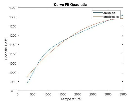
Plot2:- Quadratic polynomial curve fit

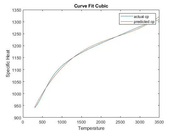
Plot3:- Cubic polynomial curve fit

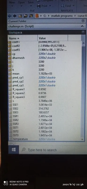
Output for getting S-square value for polynomial curve fit:-

Observation:-

1. In linear polynomial the variation is large between the curve hence the curve has not fit perfectly.
2. In quadratic polynomial the curve variation is less than compare to linear polynomial but it also not perfectly match.
3. In cubic polynomial the variations is fewer between the curve hence the curve is perfectly fit.

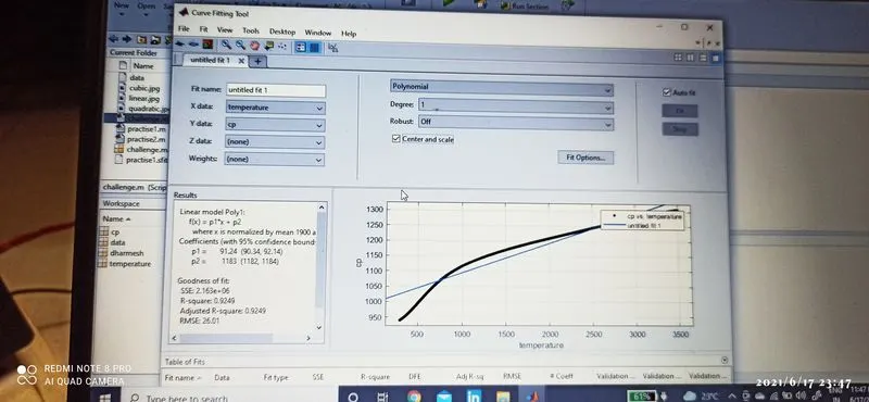
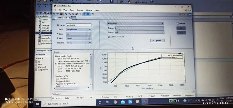
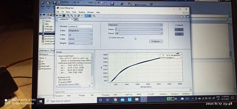
Curve fitting toolbox:- Curve fitting toolbox is another alternatiiive way to validate the fitness characteristics of the curve. We just have to prepare the data first and then open the curve fitting toolbox and then select x and y values.

Curve fitting toolbox results:-

1] Linear polynomial curve fit

2] Quadratic polynomial curve fit

3] Cubic polynomial curve fit

program on splitting data:- In this program all process is same difference is only split the data and use center and scaling in cubic polynomial using three variable in polyfit and this command [], mu in polyval.

clear all
close all
clc
%load the data
gaurav = load('data');
temp = gaurav(:,1);
cp = gaurav(:,2);

%splitting the data
temp1 = temp(1:800);
cp1 = cp(1:800);
temp2 = temp(801:1600);
cp2 = cp(801:1600);
temp3 = temp(1601:2400);
cp3 = cp(1601:2400);
temp4 = temp(2401:3200);
cp4 = cp(2401:3200);

%solve linear polynomial curve fit
[coeff1 a mu] = polyfit(temp1,cp1,1);
pred_cp1 = polyval(coeff1,temp1,[],mu);

[coeff2 a mu] = polyfit(temp2,cp2,1);
pred_cp2 = polyval(coeff2,temp2,[],mu);

[coeff3 a mu] = polyfit(temp3,cp3,1);
pred_cp3 = polyval(coeff3,temp3,[],mu);

[coeff4 a mu] = polyfit(temp4,cp4,1);
pred_cp4 = polyval(coeff4,temp4,[],mu);

%solve cubic polynomial curve fit
[coeff5 a mu] = polyfit(temp1,cp1,3);
pred_cp5 = polyval(coeff5,temp1,[],mu);

[coeff6 a mu] = polyfit(temp2,cp2,3);
pred_cp6 = polyval(coeff6,temp2,[],mu);

[coeff7 a mu] = polyfit(temp3,cp3,3);
pred_cp7 = polyval(coeff7,temp3,[],mu);

[coeff8 a mu] = polyfit(temp4,cp4,3);
pred_cp8 = polyval(coeff8,temp4,[],mu);

%plotting linear polynomial
figure(1)
plot(temp,cp,'o','color','r')
hold on
plot(temp1,pred_cp1,'color','k','linewidth',2)
plot(temp2,pred_cp2,'color','k','linewidth',2)
plot(temp3,pred_cp3,'color','k','linewidth',2)
plot(temp4,pred_cp4,'color','k','linewidth',2)
xlabel('Temperature')
ylabel('Specific Heat')
title('Curve Fit Linear')
legend('actual cp','predicted cp','location','northwest')

%plotting cubic polynomial
figure(2)
plot(temp,cp,'o','color','r')
hold on
plot(temp1,pred_cp5,'color','k','linewidth',2)
plot(temp2,pred_cp6,'color','k','linewidth',2)
plot(temp3,pred_cp7,'color','k','linewidth',2)
plot(temp4,pred_cp8,'color','k','linewidth',2)
xlabel('Temperature')
ylabel('Specific Heat')
title('Curve Fit Cubic')
legend('actual cp','predicted cp','location','northwest')

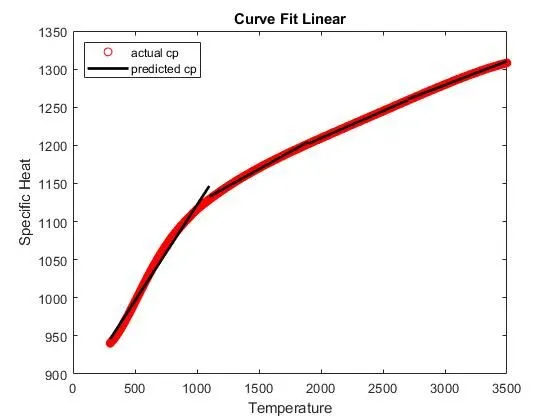
Plot1:- Linear polynomial curve fit

Plot2:- Cubic polynomial curve fit

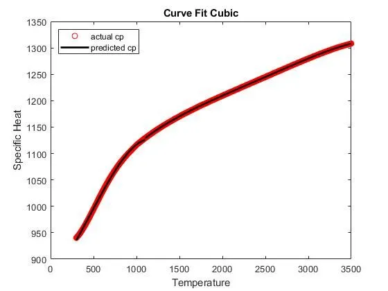
Observation:- In linear polynomial create small variations so its not fit to curve and in cubic polynomial no variations are created so its perfecftly fit. creating split data in cubic polynomial gives better result.

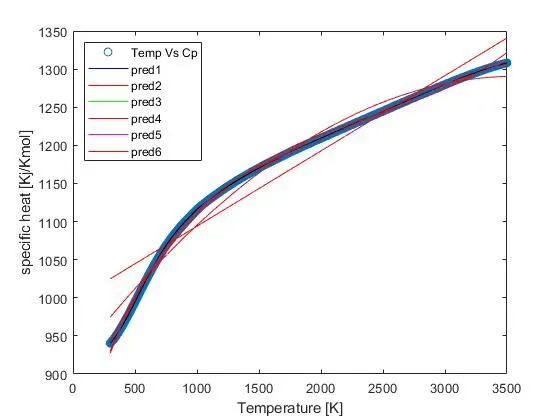
Program:- In this program we use two new commands 1st gof it mean goodness of fit statistic and 2nd is normalise its use for centering and scaling.

clear all
close all
clc

a = load('data');
temp = a(:,1);
cp = a(:,2);


[pred1 gof] = fit(temp,cp,'poly1')
pred2 = fit(temp,cp,'poly2','Normalize','on')
pred3 = fit(temp,cp,'poly3','Normalize','on')
pred4 = fit(temp,cp,'poly4','Normalize','on')
pred5 = fit(temp,cp,'poly5','Normalize','on')
pred6 = fit(temp,cp,'poly6','Normalize','on')


plot(temp,cp,'o')
hold on
plot(pred1,temp,cp,'b')
plot(pred2,temp,cp,'g')
plot(pred3,temp,cp,'m')
plot(pred4,temp,cp,'k')
plot(pred5,temp,cp,'c')
plot(pred6,temp,cp,'k')
xlabel('Temperature [K]')
ylabel('specific heat [Kj/Kmol]')
legend('Temp Vs Cp','pred1','pred2','pred3','pred4','pred5','pred6')

Plot:-

Question and answer:-

1. How to make a curve fit perfectly?

Ans :- To find the R-square value and R-square value must be equal to one then the curve fit will be perfect.

2. How to get the best fit?

Ans :- When we split the values and plot the curve then get best fit curve. Also finding the R-square value, it should be greater than 0.95 then the assumed fit is good.

3. What could be done to improve the cubic fit?

Ans :- For improving the cubic fit we have to split the values of given data into set of values so improving cubic fit and it will reduces the warning symbol.

Conclusion:- There are many methods use for to make curve fit properly, we need to have high order polynomial eqn to achieve the perfect fit, and by splitting data we get better fit, more the number of splits they gave better the output result.

Thank you

Dharmesh bonde