Simulation of simple pendulum by solving second order ODE using matlab

Write a program in MATLAB/OCTAVE that will simulate the pendulum motion by second order ordinary differential equation.

Introduction:-

In a simply language pendulum is a object that has small mass also known as bob which is suspended from a wire or string of negligible mass.When displaced a pendulum will ocillate around its equilibrium point due to momentum in balance with the restoring force of gravity.

It consist mass M hanging from a string of length L and fixed at pivot point P.when displaced to an initial angle is Theta. Its working principle is Newtons second law for rotational system.

Theory:-

For this simulation of pendulum motion by second order ordinary differential equation. This ODE represents the equation with damping

`frac{d^2theta}{dt^2}+frac{b}{m}frac{d theta}{dt}+frac{g}{l}sin theta=0`

Where, g = Gravity in (m/s^2),

l = length of pendulum (m),

m = mass of the ball (kg),

b = damping coefficient.

now convert the second order ordinary differential equation into first order ordinary differential equation because second order ordinary differential equation is cannot solved by matlab so conversion is must required.

`frac{d^2theta}{dt^2}+frac{b}{m}.frac{d theta}{dt}+frac{g}{l}sin theta=0`....................[1]

Let us consider,

`theta = theta1`...........[2]

`frac{d theta}{dt}`...........[3]

substitute equation 2 into 3

`frac{d theta1}{dt}`...........[4]

theta1 change wrt time

`frac{d theta1}{dt}=theta2`...........[5]

`frac{d^2theta}{dt^2}`..........[6]

substitute equation 1 into 6

`frac{d^2theta1}{dt^2}`..........[7]

solving equation 7

`frac{d}{dt}(frac{d theta1}{dt})`........[8]

substitute equation 5 into 8

`frac{d}{dt}(theta2)`.........[9]

now will substitute eqn 5 and 8 into 1

`frac{d}{dt}(frac{d theta1}{dt})+frac{b}{m}*theta2+frac{g}{l}*sintheta1=0`.........10

substitute eqn 9 into 10

`frac{d}{dt}(theta2)+frac{b}{m}*theta2+frac{g}{l}*sintheta1=0`

`frac{d theta2}{dt}=-(frac{b}{m})*theta2-(frac{g}{l})*sintheta1`

by using above eqn we create first order now will simulate pendulum using MATLAB

Process:-

1. Firstly consider theta1 as theta(2) as using above equations and same as theta2.
2. convert the second order ordinary differential equation into first order ordinary differential equation.
3. create matrix.
4. give function, the function name is same as file name.

function [dtheta_dt] = challenge(t,theta,b,m,g,l)

theta1 = theta(1)
theta2 = theta(2)

%conversion 1st ode
dtheta1 = theta2;
dtheta2 = -(b/m)*theta2-(g/l)*sin(theta1);

dtheta_dt = [dtheta1;dtheta2];
end

Process:-

1. Start to main program using clear all, close all and clc command.
2. Put given parameters in program.
3. Then we called above function code .
4. solve differential equation using ode45 command.
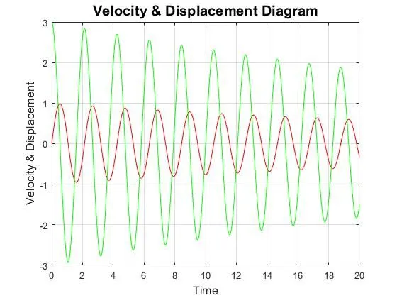
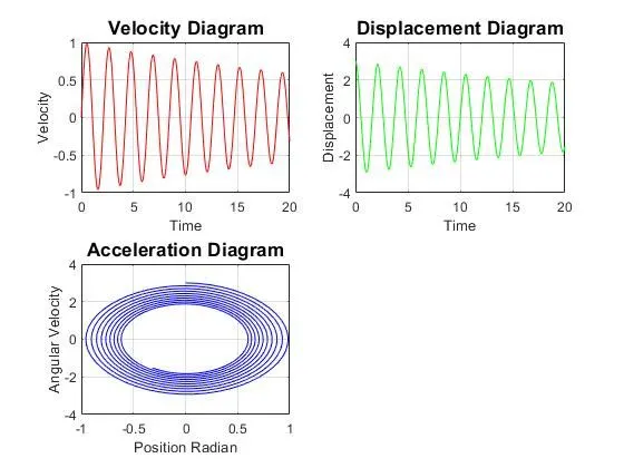
5. then we create a plot 1) velocity and displacement vs time, 2) velocity vs time, 3) displacement vs time, 4) angular velocity and acceleration in same figure using subplot command.
6. then we create animation of pendulum for time span using this commands getframe, movie, contour.

clear all
close all
clc

%inputs
b = 0.05;   %damping coefficient
m = 1;      %mass of bob
g = 9.81;   %garvitational force
l = 1;      %length of string

%initial condition
theta_0 = [0;3];

%time points
t_span = linspace(0,20,500);

%ode45 solving
[t,results] = ode45(@(t,theta)challenge(t,theta,b,m,g,l),t_span,theta_0)

%plotting
%velocity & displacement vs time diagram
figure(1)
plot(t,results(:,1),'color','r')
hold on
plot(t,results(:,2),'color','g')
hold off
xlabel('Time','fontsize',12)
ylabel('Velocity & Displacement','fontsize',12)
title('Velocity & Displacement Diagram','fontsize',15)
grid on

figure(2)
%velocity vs time diagram
subplot(2,2,1)
plot(t,results(:,1),'color','r')
xlabel('Time','fontsize',10)
ylabel('Velocity','fontsize',10)
title('Velocity Diagram','fontsize',13)
grid on

%displacent vs time diagram
subplot(2,2,2)
plot(t,results(:,2),'color','g')
xlabel('Time','fontsize',10)
ylabel('Displacement','fontsize',10)
title('Displacement Diagram','fontsize',13)
grid on

%acceleration diagram
subplot(2,2,3)
plot((results(:,1)),(results(:,2)),'color','b')
xlabel('Position Radian','fontsize',10)
ylabel('Angular Velocity','fontsize',10)
title('Acceleration Diagram','fontsize',13)
grid on

%for animation
theta3 = results(:,1)
ct = 1;
for i = 1:length(theta3)
T3 = theta3(i)

%coordinates
x0 = 0;
y0 = 0;

x1 = l*sin(T3);
y1 = -(l*cos(T3));

%plotting for animation
figure(3)
plot([-1 1],[0 0],'linewidth',5,'color','k')   %create line which is connected to string through pivot
hold on
plot([0 0],[0 0],'o','markerfacecolor','g','markersize',20)  %create pivot 
line([x0 x1],[y0 y1],'linewidth',5,'color','r')  %create string
plot(x1,y1,'o','markerfacecolor','b','markersize',50) %create bob
hold off
axis([-1.5 1 -1.5 1])
pause(0.02)
A(ct) = getframe(gcf)
ct = ct+1;
end

% create movie
movie(A)
videofile = VideoWriter('dharmesh.avi','Uncompressed AVI')
open(videofile)
writeVideo(videofile,A)
close(videofile)

Figures:-

• velocity and displacement vs time:-

• 1) velocity vs time, 2) displacement vs time, 3) angular velocity and acceleration:-

• Animated pendulum:-

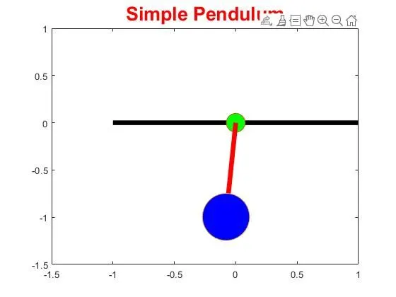
Observation:- By observing above figure movement is softly.

Result:- When time increases dispacement and velocity are decreases because of damping coefficient.

Video link:-

https://youtu.be/WFjAPo0HKrg

Thank you,

Dharmesh Bonde