Week 9- Simulate the motion of blades in a generic turbomachinery component using an unsteady moving zone approach
Objective:
Simulate the motion of blades in a generic turbomachinery component using an unsteady approach.
- Assume blade rotation at 300rpm
- Choose an appropriate time step for the simulation and generate an animation file for the rotation.
Answer:
The project is about the simulating of generic turbomachinery ccomponent under no load conditions with 2 different conditions, one is Moving Reference Frame (MRF) & Moving Mesh approach.
No. of blades/airfoils = 10
Blades' angular velocity = 250 rpm
Chord length of blade = 0.6m
Angle between 2 blades = 36 degree
Flow condition = Turbulent (assumed)
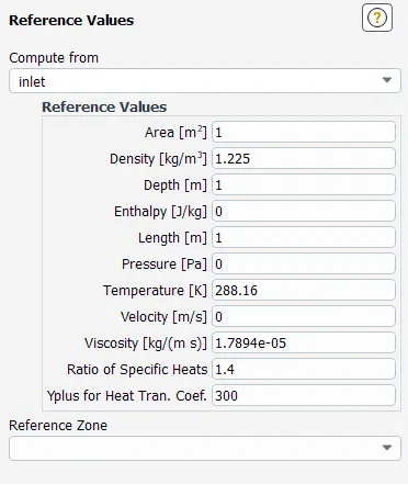
Inlet & outlet are at ambient conditions.
The MRF (Moving Reference Frame) approach has been simiulated in steady state condition while, Moving mesh approach in unsteady state condition.
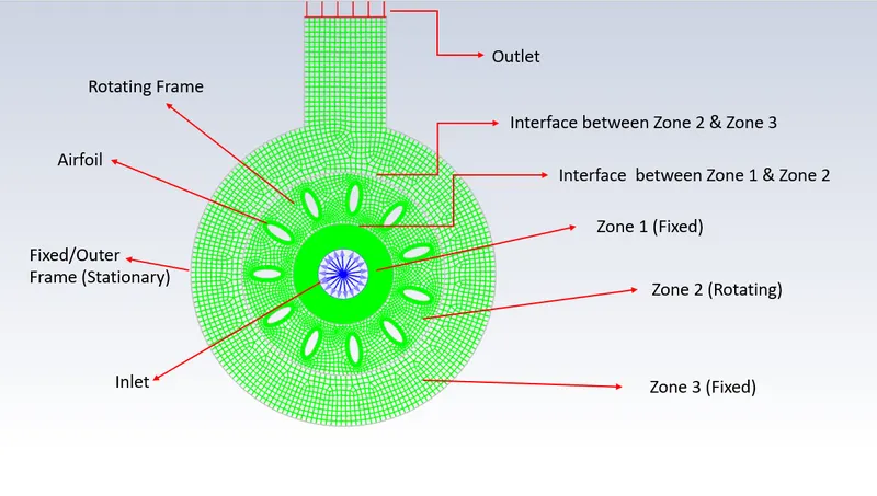
Different parts are defined in below image for the reference.
As it can be seen that zone 1 is comprised of inlet while zone 2 & 3 are comprised of rotating frame & outer fixed frame respectively.
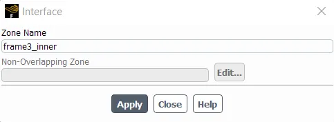
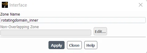
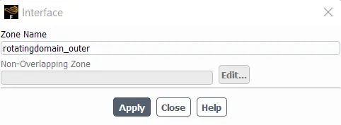
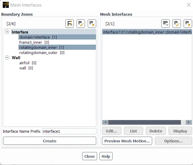
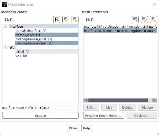
To transfer data, interface between zone 1 & 2 and zone 2 & 3 will be set up.
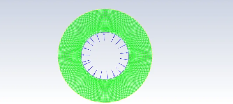
The geometry has been given as three seperate parts which will be joined inside the Ansys Fluent software by using the option called "appending files". Following is the domain 1 which is inserted through import mesh option.
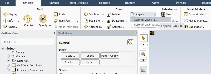
Following option has been used to apprehend next 2 domain.
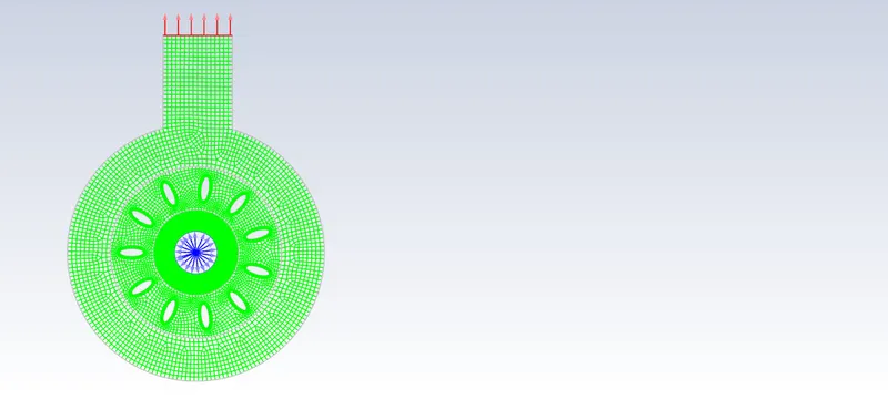
Final geometry after joining all three domains is shown in below image.
Carse 1: Moving reference Frame Approach (Steady State Simulation)
Simulation Setup:
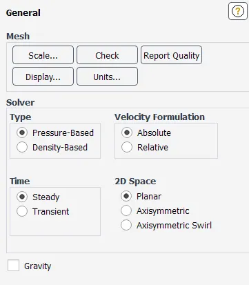
Viscous Model:
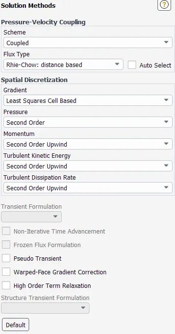
For internal flow & turbomachinery flows, k-epsilon Realizable model is very well proven model for the accurate results.
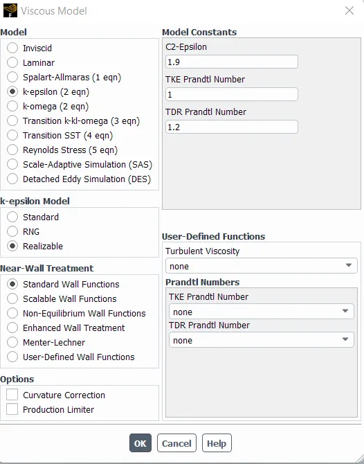
Material:
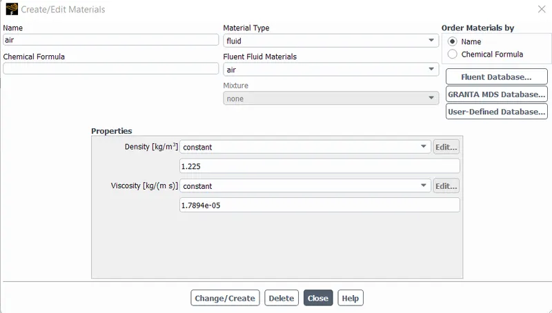
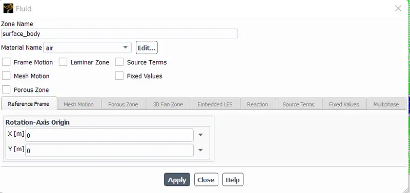
Cell zone conditions:
Fixed frame = zone 1
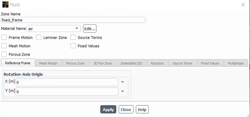
Rotating frame = zone 2
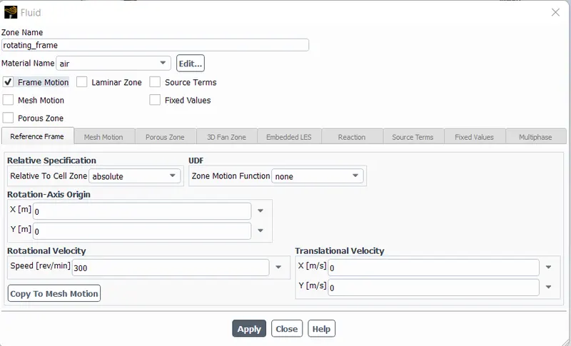
Surface body = zone 3
Boundary Conditions:
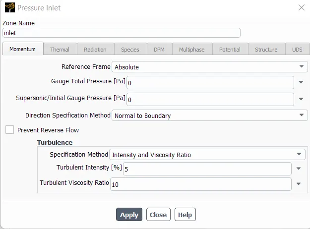
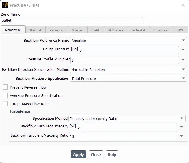
To create "No Load Condition", the inlet & outlet was kept at same pressure level. And inlet is assigned as pressure-inlet.
Inlet
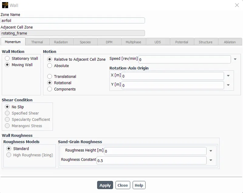
Airfoil has been set as Moving wall with Relative to adcent Cell Zone motion condition because the cell zone of rotary frame is already defined for Moving Frame approach with 300 rpm angular velocity.
Mesh Interface:
Reference Values:
Solution Methods:
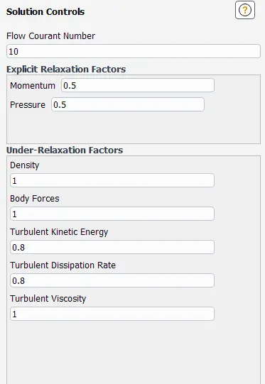
Solution Controls:
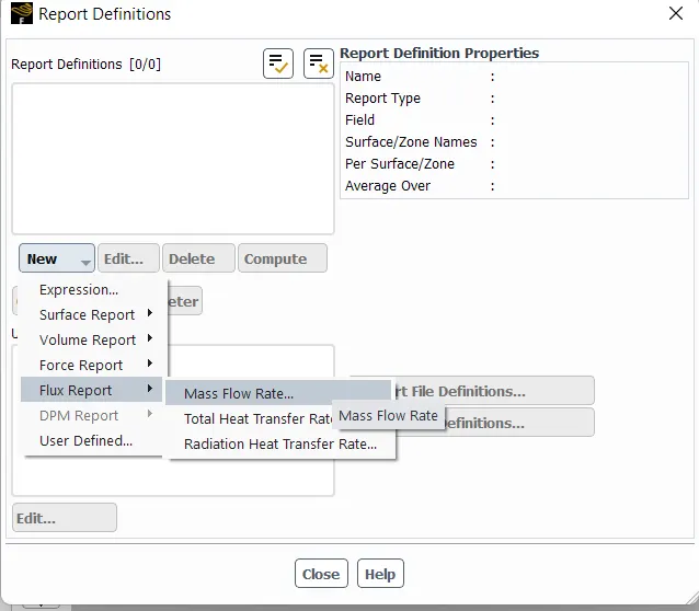
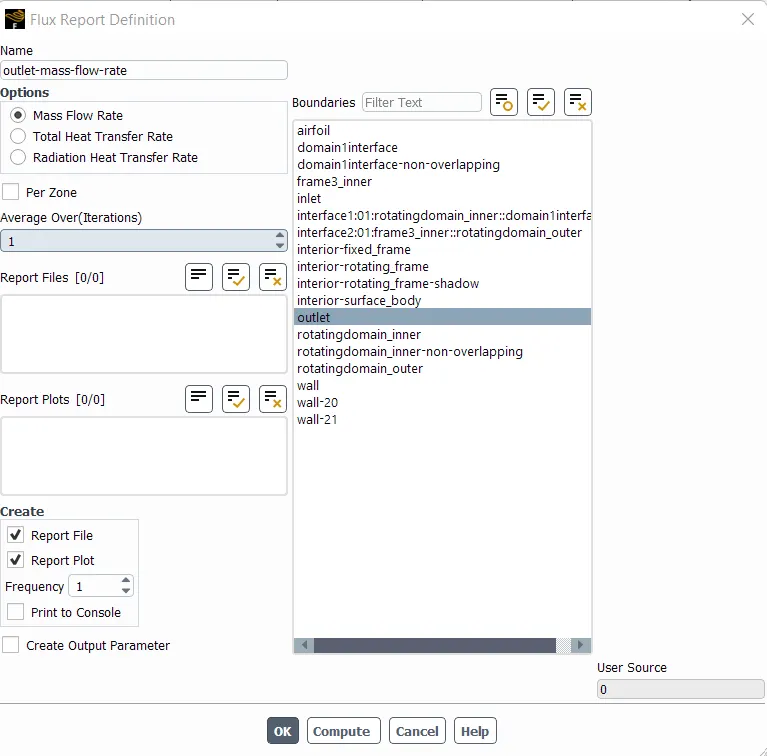
Report Definition:
1. Mass Flow Rate - Outlet
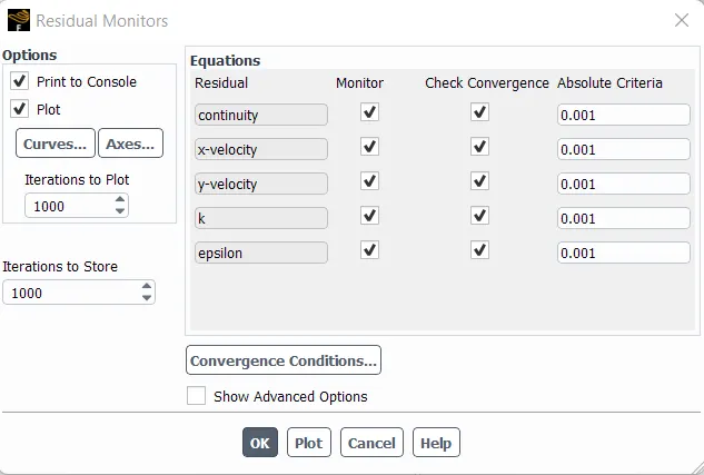
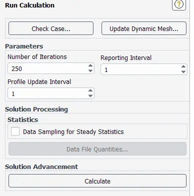
Residuals:
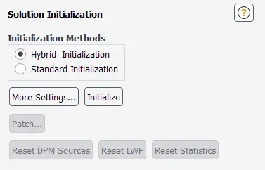
Initialization
Results:
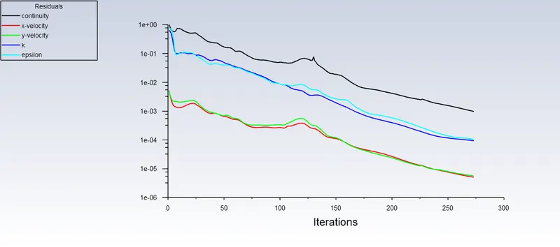
Residual plot
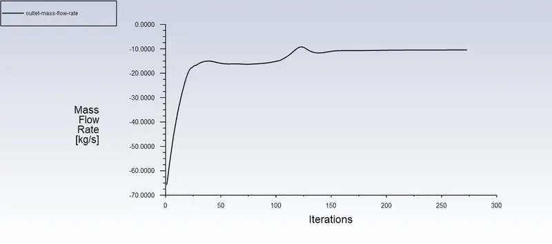
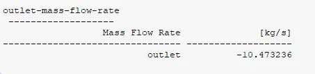
Mass Flow Rate
Velocity Contour
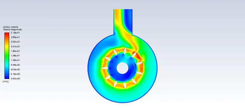
In velocity contour plot, it can be seen that area near by the most outer edge has the lowest velocity while the area surrounded by the airfoils have the highest velocity.
Animation
Vorticity Contour
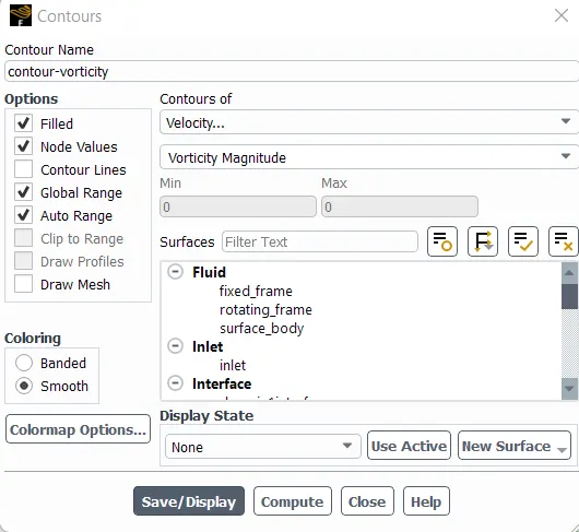
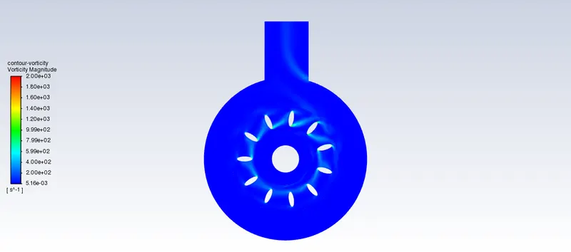
Using this plot, we can visualize from where the flow would have dettached.
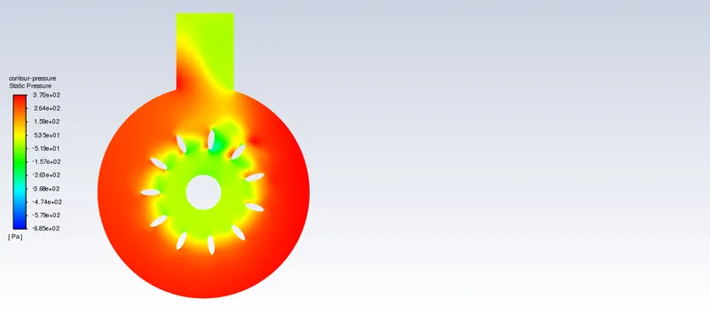
Pressure Contour
XY Plots
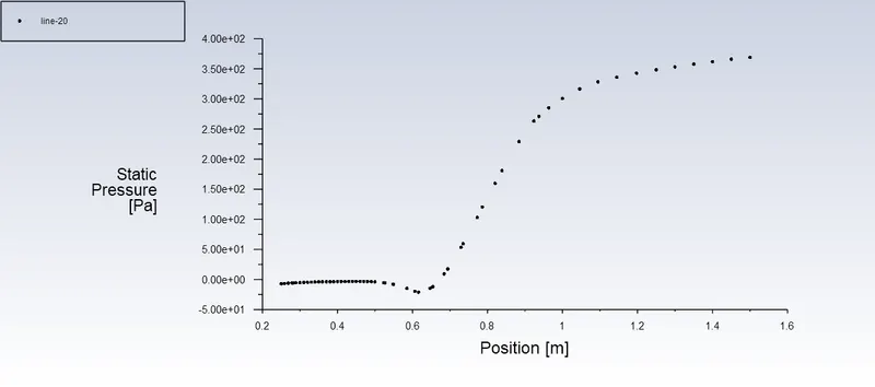
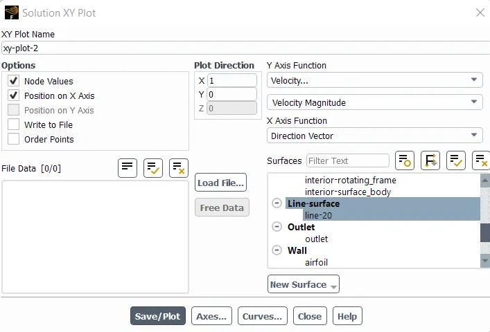
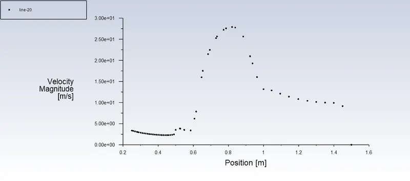
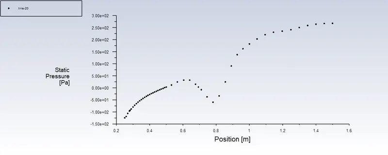
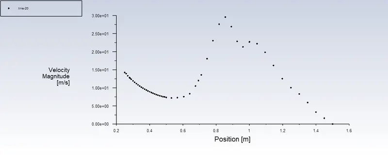
Line has been created across the component in X-direction to plot the graph using following options.
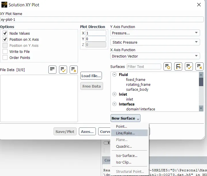
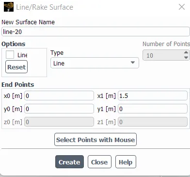
For Pressure
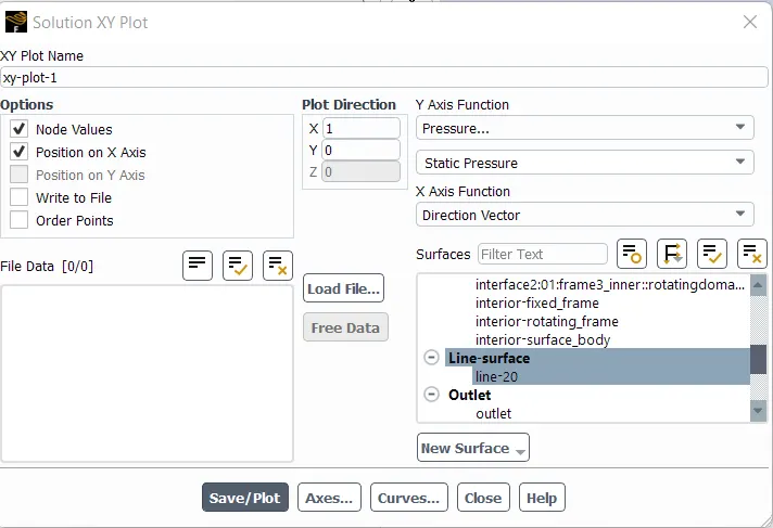
For Velocity
Case 2: Moving Mesh Approach - Unsteady State Condition
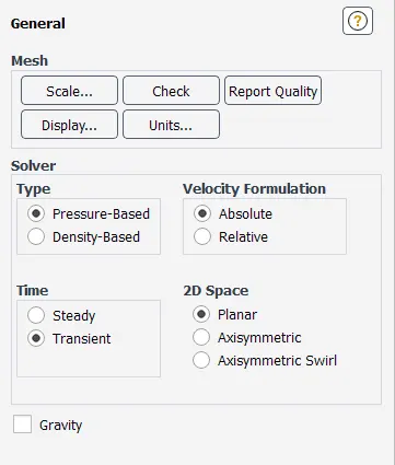
The steps which are not similar to the steady state conditions have been displayed in below images.
Transient Condition
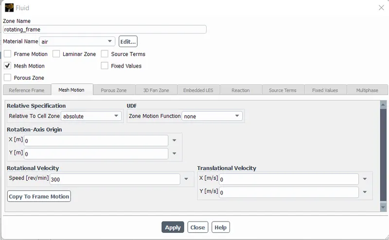
Cell Zone conditions:
Applying Moving Mesh approach using "Mesh Motion".
Boundary Conditions:
- In the Moving mesh approach, normally the interfaces between zones are not required to assigned. But as the component is divided into multiple zones, we need to follow the interface assigning steps & mesh interface step for this approach as well.
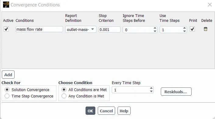
Convergence Conditions:
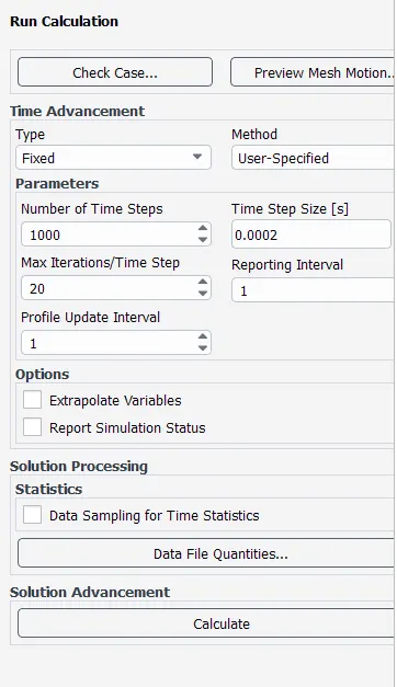
Calculation for Time Step size:
Given Rotational velocity (N) = 300 RPM
Angular velocity, `omega = (2piN)/60 = (2pi)/T`
So, for time period, T = 60/N = 60/300 = 0.2 sec
So, to achieve this time period in 1000 time steps than
Time Step size (`DeltaT`) = T/1000 = 0.2/1000 = 0.0002
Results:
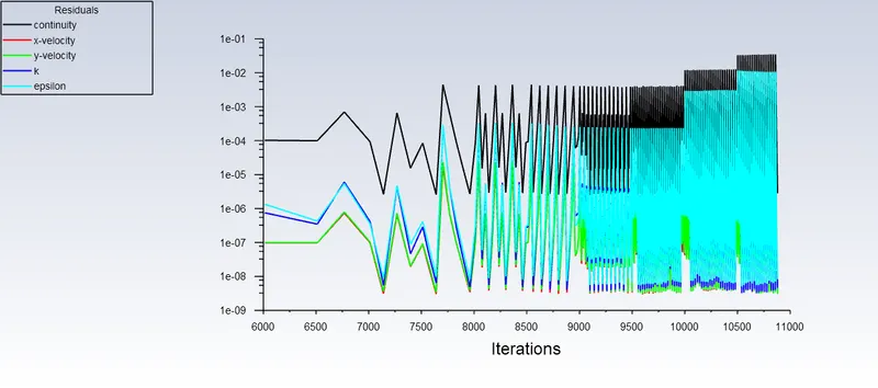
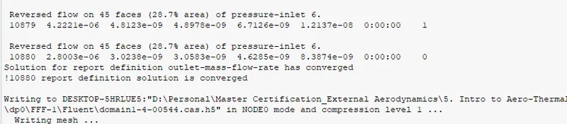
Residual plot
Mass Flow Rate:
Velocity Contour
Animation - Velocity Contour
Vorticity Contour
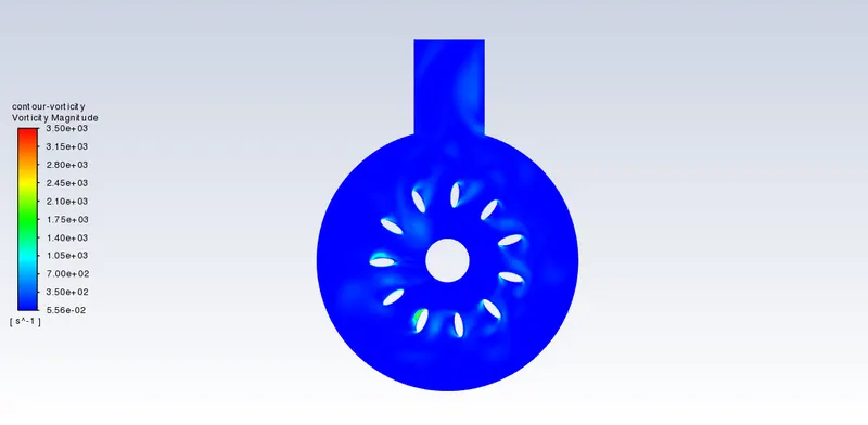
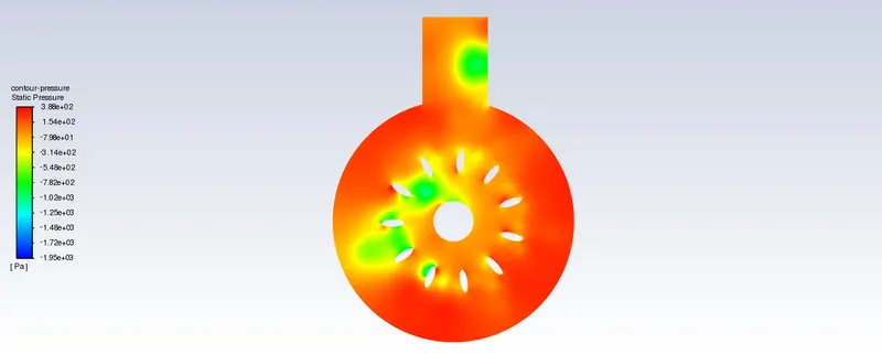
Pressure Contour
Pressure Distribution along horizontal line
Velocity magnitude along horizontal line
Comparision between two approaches:
| Velocity (m/s) | Pressure (Pa) | Condition | Mass Flow Rate (kg/s) | |
| Moving Frame Approach | 31.6 | 37 | Steady State | -10.47 |
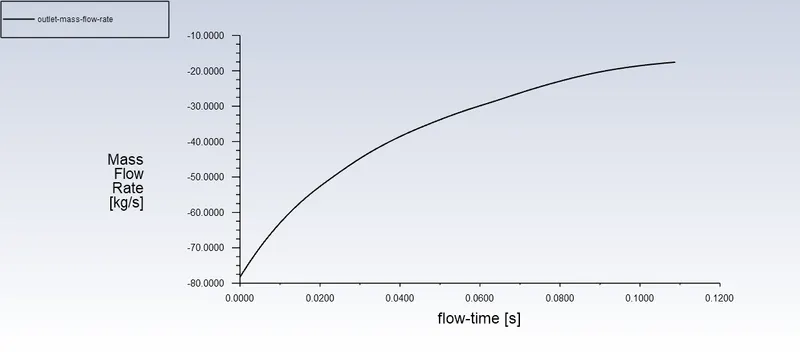
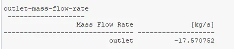
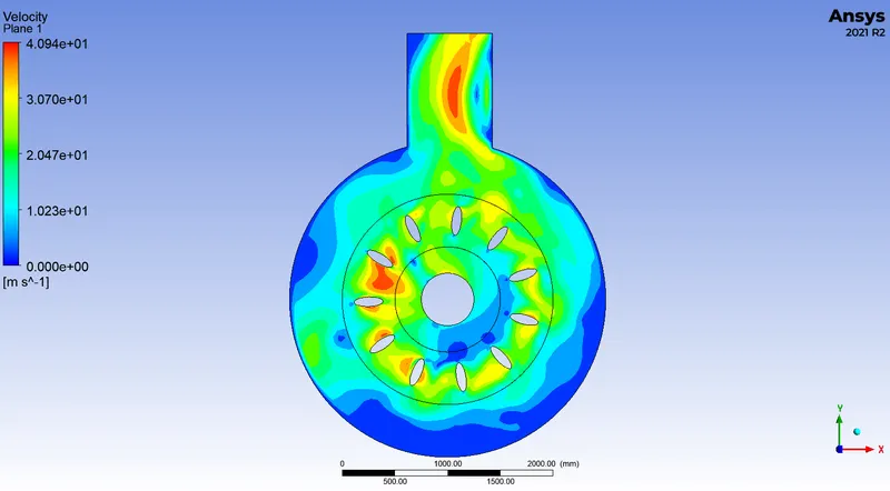
| Moving Mesh Approach | 40.94 | 38.8 | Transient | -17.57 |
from the above table, it can be observed that the velocity, pressure & mass flow rate obtained in Moving Mesh approach is more than the Moving reference frame approach.