Simulating a 2nd order ODE system of a Simple Pendulum equation

The second order ODE for the Simple Pendulum Motion with Damping is as follows:

`(d^2theta)/dt^2 + (b/m) * (d theta)/(dt) + g/l*sin theta = 0`

The equation has second order derivative involved, because of that equation is required to convert into two first order equation to solve using the MATLAB function.

Following variable has been introduced:

`theta`= `theta1`

`(d theta)/dt = (d theta1)/dt = theta2`

&

`(d^2 theta)/dt^2 = d/dt((d theta)/dt) = d/dt((d theta1)/dt) = d/dt*theta2`

Inserting, values of variables into the main equation,

`(d theta2)/dt + b/m * theta 2 + g/l * sin theta1 = 0`

`(d theta2)/dt = - (b/m * theta2) - (g/l * sin theta1)`

Putting them into matrix form

`d/dt [ [theta1], [theta2]] = [[theta2], [-(b/m)*theta2 - (g/l)*sin theta1]]`

Two equations mentioned in the matrix form will be used to create the animation of the simple pendulum with damping effect using in- built ODE45 MATLAB solver.

Main Code:

% Pendulum Animation Program

% Objective: Writing the program to animate the pendulum motion for 20
% seconds according to given inputs. The program required to solve the
% second order ODE that represents the simple pendulum motion with damping using the
% ODE45 in-built MATLAB function. Two graphs also reqiored to plot, each
% for angular displacement & angular velocity against time. 

% Inputs: 
% Gravity(g) = 9.81 m/s^2
% Length of the pendulum (L) = 1 meter
% mass of the ball (m) = 1 kg
% Damping Coefficinet (b) = 0.05
% time span = 20 seconds
% Initial condition, at t=0, angular displacement = 0 & angular velocity =
% 3 rad/s

% Second order ODE representing the pendulum motion with damping 
% (d^2(theta)/(d(theta))^2) + (b/m)(d(theta)/dt) + (g/L)sin(theta) = 0

% To solve this equation in MATLAB using ODE45 function, the equation needs
% to be converted into the two first order ODE by using new variables

% The new variable, theta = theta(1) has been introduced.
% Two new first order ODEs are:
% d(theta)/dt = theta(2)
% d(theta(2))/dt = -(b/m)*theta(2) - (g/L)*sin(theta(1))

clc; clear all; close all;

% Design Inputs
L = 1;  % Length of Pendulum (meter)

% Time Span
t_end = 20; % Total Duration (s)

% Defining initial & Total Time Duration
t = [0 t_end];

% Angular Displacement & Angular Velocity = Initial Condition
theta_0 = [0 3]; % [rad rad/s]

% Solving Pendulum ODE using ODE45
% ODE45 function solves the nonstiff differential equations. It performs a
% direct numerical integration of set of differential equations in the form
% of y' = f(t,x)

[t, theta] = ode45('Pendulum_eqn', t, theta_0);

% Converting Position Cylindrical to Cartesian Coordinates
% cartesian_cord = [L*sin(theta(:,1)) L*cos(theta(:,1))];

% Converting Angular Velocity to Linear Velocity in X & Y 
% velocity = [L*theta(:,2).*cos(theta(:,1)) L*theta(:,2).*sin(theta(:,1))];

% Plotting Results for Angular Displacement & Angular Velocity
figure(1)

% To create two plots in one plot, subplot function has been used
subplot(2,1,1) % For Angular Displacement
plot(t,theta(:,1), 'Linewidth', 1.5)
ylabel('Angular Displacement (rad)', 'FontSize', 7);
title('Angular Displacement vs Time');
grid on
ax = gca; ax.FontSize = 9; % Changing fontsize of graph axis labels

subplot(2,1,2) % Angular Velocity
plot(t,theta(:,2), 'LineWidth', 1.5)
xlabel('Time(Seconds)', 'FontSize', 7)
ylabel('Angular Velocity (rad/sec)', 'FontSize', 7)
title('Angular Velocity vs Time');
grid on
ax = gca; ax.FontSize = 9; 

% Creating Pendulum Animation
counter_var = 1; % Creating counter variable to capture the pendulum motion in frames
for i = 1:length(theta)
    theta_values = theta(i,1) 
    
    % Initial position of pendulum
    x_initial = 0;
    y_initial = 0;
    
    % Converting Position Cylindrical to Cartesian Coordinates
    x_1 = L*sin(theta_values);
    y_1 = -L*cos(theta_values);
    
    % Creating the Pendulum figure
    figure(2)
    
    % Creating marker which replicate the Pendulum ball
    plot(x_1, y_1, 'o', 'markersize', 25, 'markerfacecolor', 'k')
    
    hold on % hold command will help to plot all points individually
    
    % Creating strings that replicate the pendulum 
    plot([x_initial x_1],[y_initial y_1])
    
    plot([-0.5 0.5],[0 0]) % Graph Size
    axis([-1.5 1.5 -2 0.5]) % Axis size
    
    % Writing Title of the animation in multiple lines
    title({'Simple Pendulum Motion',['Time: ', num2str(t(i))]});
    
    pause (0.02) % To slow down the video speed
    hold off
    
    % getframe(gcf) command will help to capture all the latest images and
    % all images will be saved in the M(counter_var) variable.
    % Incrementing counter_var will help to collect all the images which
    % will be used to create animation.
    M(counter_var) = getframe(gcf); 
    counter_var = counter_var + 1;
end

 % Stitching all images together to form animation animation using "movie"
 % function
movie(M)

% VideoWriter function will be used to create uncompressed animation file
animation = VideoWriter('Pendulum_Animation.avi','Uncompressed AVI');

open(animation)
writeVideo(animation, M)
close(animation)

Function:

function [theta_dot] = Pendulum_eqn(t,theta)

% Funcion file for the Pendulum challenge 

% Writing function to insert into the ODE45 function to calculate the
% movement of the pendulum. The Pendulum equation has been converted into
% the two first derivative equation from the second order pendulum
% equation. 

% Design Inputs
L = 1;  % Length of Pendulum (meter)
m = 1;  % Mass of the Pendulum (kg)
b = 0.05;   % Damping Coefficient
g = 9.81; % Gravity (m/s^2)

% creating matrix to store the values of the theta_dot(1) and theta_dot(2)
% values
theta_dot = zeros(2,1); 

% Inserting the first order ODEs of the Simple Pendulum Motion equations
theta_dot(1) = theta(2); % First Derivative 
theta_dot(2) = - (b/m)*theta(2) - (g/L)*sin(theta(1)); % Second Derivative

end

Results:

1. Graphs

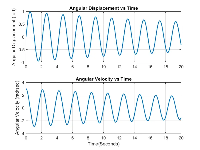
2. Pendulum Animation Video

https://youtu.be/qLs0kqxSki8